Traditional or robust variogram methods for spatial data
vgram.Rdvgram computes pairwise squared differences as a function of distance.
Returns an S3 object of class "vgram" with either raw values or statistics from
binning. crossCoVGram is the same as vgram but differences are
taken across different variables rather than the same variable.
plot.vgram and boxplotVGram create lineplots and boxplots of
vgram objects output by the vgram function. boxplotVGram plots
the base R boxplot function, and plots estimates of the mean over the boxplot.
The getVGMean function returns the bin centers and means of the vgram
object based on the bin breaks provided by the user.
vgram(loc, y, id = NULL, d = NULL, lon.lat = FALSE,
                    dmax = NULL, N = NULL, breaks = NULL,
                    type=c("variogram", "covariogram", "correlogram"))

crossCoVGram(loc1, loc2, y1, y2, id = NULL, d = NULL, lon.lat = FALSE,
                        dmax = NULL, N = NULL, breaks = NULL,
                        type=c("cross-covariogram", "cross-correlogram"))

boxplotVGram(x, N=10, breaks = pretty(x$d, N, eps.correct = 1), plot=TRUE, plot.args, ...)

# S3 method for vgram
plot(x, N=10, breaks = pretty(x$d, N, eps.correct = 1), add=FALSE, ...)

getVGMean(x, N = 10, breaks = pretty(x$d, N, eps.correct = 1))
Arguments
- loc
Matrix where each row is the coordinates of an observed point of the field
- y
Value of the field at locations
- loc1
Matrix where each row is the coordinates of an observed point of field 1
- loc2
Matrix where each row is the coordinates of an observed point of field 2
- y1
Value of field 1 at locations
- y2
Value of field 2 at locations
- id
A 2 column matrix that specifies which variogram differnces to find. If omitted all possible pairing are found. This can used if the data has an additional covariate that determines proximity, for example a time window.
- d
Distances among pairs indexed by id. If not included distances from from directly from loc.
- lon.lat
If true, locations are assumed to be longitudes and latitudes and distances found are great circle distances (in miles see rdist.earth). Default is FALSE.
- dmax
Maximum distance to compute variogram.
- N
Number of bins to use. The break points are found by the
prettyfunction and so ther may not be exactly N bins. Specify the breaks explicity if you want excalty N bins.- breaks
Bin boundaries for binning variogram values. Need not be equally spaced but must be ordered.
- x
An object of class "vgram" (an object returned by
vgram)- add
If
TRUE, adds empirical variogram lineplot to current plot. Otherwise creates new plot with empirical variogram lineplot.- plot
If
TRUE, creates a plot, otherwise returns variogram statistics output bybplot.xy.- plot.args
Additional arguments to be passed to
plot.vgram.- type
One of "variogram", "covariogram", "correlogram", "cross-covariogram", and "cross-correlogram".
vgramsupports the first three of these andcrossCoVGramsupports the last two.- ...
Additional argument passed to
plotforplot.vgramor tobplot.xyforboxplotVGram.
Value
vgram and crossCoVGram return a "vgram" object containing the
following values:
- vgram
Variogram or covariogram values
- d
Pairwise distances
- call
Calling string
- stats
Matrix of statistics for values in each bin. Rows are the summaries returned by the stats function or describe. If not either breaks or N arguments are not supplied then this component is not computed.
- centers
Bin centers.
If boxplotVGram is called with plot=FALSE, it returns a
list with the same components as returned by bplot.xy
References
See any standard reference on spatial statistics. For example Cressie, Spatial Statistics
See also
Examples
#
# compute variogram for the midwest ozone field day 16
# (BTW this looks a bit strange!)
#
data( ozone2)
good<- !is.na(ozone2$y[16,])
x<- ozone2$lon.lat[good,]
y<- ozone2$y[16,good]
look<-vgram( x,y, N=15, lon.lat=TRUE) # locations are in lon/lat so use right
#distance
# take a look:
plot(look, pch=19)
 #lines(look$centers, look$stats["mean",], col=4)
brk<- seq( 0, 250,, (25 + 1) ) # will give 25 bins.
## or some boxplot bin summaries
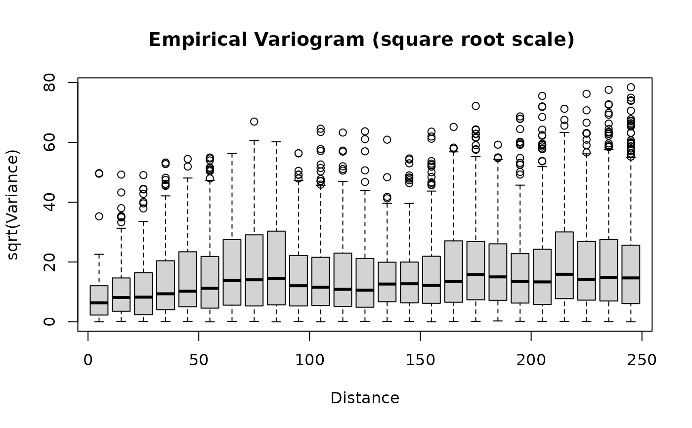
boxplotVGram(look, breaks=brk, plot.args=list(type="o"))
plot(look, add=TRUE, breaks=brk, col=4)
#lines(look$centers, look$stats["mean",], col=4)
brk<- seq( 0, 250,, (25 + 1) ) # will give 25 bins.
## or some boxplot bin summaries
boxplotVGram(look, breaks=brk, plot.args=list(type="o"))
plot(look, add=TRUE, breaks=brk, col=4)
 #
# compute equivalent covariogram, but leave out the boxplots
#
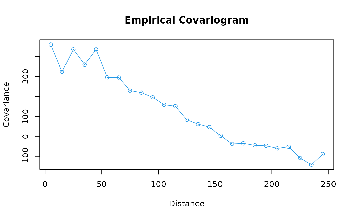
look<-vgram( x,y, N=15, lon.lat=TRUE, type="covariogram")
plot(look, breaks=brk, col=4)
#
# compute equivalent covariogram, but leave out the boxplots
#
look<-vgram( x,y, N=15, lon.lat=TRUE, type="covariogram")
plot(look, breaks=brk, col=4)
 #
# compute equivalent cross-covariogram of the data with itself
#(it should look almost exactly the same as the covariogram of
#the original data, except with a few more points in the
#smallest distance boxplot and points are double counted)
#
look = crossCoVGram(x, x, y, y, N=15, lon.lat=TRUE, type="cross-covariogram")
plot(look, breaks=brk, col=4)
#
# compute equivalent cross-covariogram of the data with itself
#(it should look almost exactly the same as the covariogram of
#the original data, except with a few more points in the
#smallest distance boxplot and points are double counted)
#
look = crossCoVGram(x, x, y, y, N=15, lon.lat=TRUE, type="cross-covariogram")
plot(look, breaks=brk, col=4)
