library(fields)
#> Loading required package: spam
#> Spam version 2.9-1 (2022-08-07) is loaded.
#> Type 'help( Spam)' or 'demo( spam)' for a short introduction
#> and overview of this package.
#> Help for individual functions is also obtained by adding the
#> suffix '.spam' to the function name, e.g. 'help( chol.spam)'.
#>
#> Attaching package: 'spam'
#> The following objects are masked from 'package:base':
#>
#>     backsolve, forwardsolve
#> Loading required package: viridis
#> Loading required package: viridisLite
#>
#> Try help(fields) to get started.
1. Tps
1.1. First
str(ChicagoO3)
#> List of 3
#>  $ x      : num [1:20, 1:2] 10.24 3.8 9.11 9.62 -2.43 ...
#>   ..- attr(*, "dimnames")=List of 2
#>   .. ..$ : chr [1:20] "170310032" "170310037" "170310050" "170311002" ...
#>   .. ..$ : chr [1:2] "East.West" "North.South"
#>  $ y      : num [1:20] 36.5 34.6 31.6 34.5 37.7 ...
#>  $ lon.lat: num [1:20, 1:2] -87.5 -87.7 -87.6 -87.6 -87.8 ...
#>   ..- attr(*, "dimnames")=List of 2
#>   .. ..$ : chr [1:20] "170310032" "170310037" "170310050" "170311002" ...
#>   .. ..$ : chr [1:2] "lon" "lat"

# 2-d example
fit <- Tps(ChicagoO3$x, ChicagoO3$y) # fits a surface to ozone measurements.

set.panel(2, 2)
#> plot window will lay out plots in a 2 by 2 matrix
plot(fit) # four diagnostic plots of  fit and residuals.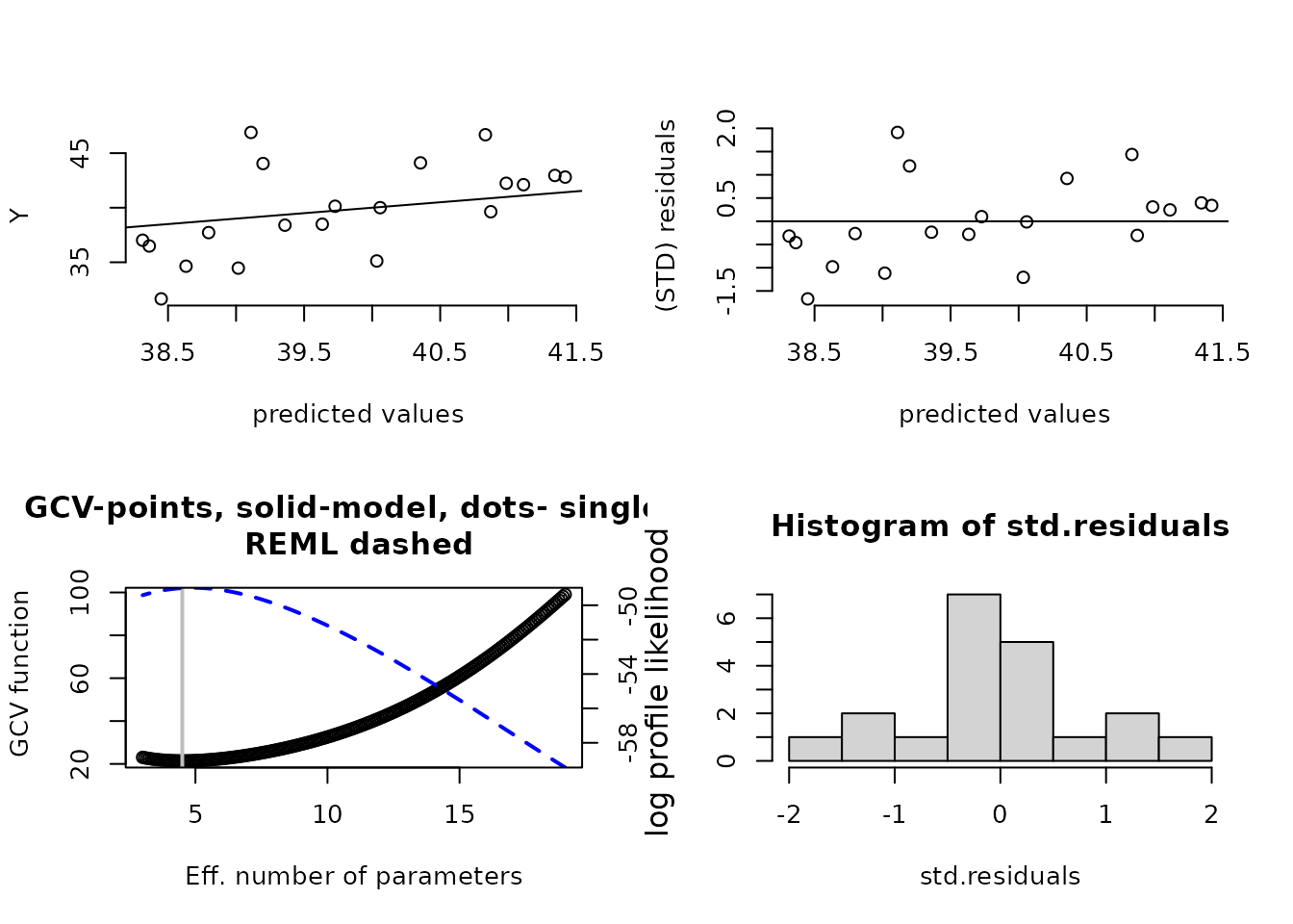
set.panel()
#> plot window will lay out plots in a 1 by 1 matrix

# summary of fit and estiamtes of lambda the smoothing parameter
summary(fit)
#> CALL:
#> Tps(x = ChicagoO3$x, Y = ChicagoO3$y)
#>
#>  Number of Observations:                20
#>  Number of unique points:               20
#>  Number of parameters in the null space 3
#>  Parameters for fixed spatial drift     3
#>  Effective degrees of freedom:          4.5
#>  Residual degrees of freedom:           15.5
#>  MLE tau                                3.779
#>  GCV tau                                4.073
#>  MLE sigma                              347.7
#>  Scale passed for covariance (sigma)    <NA>
#>  Scale passed for nugget (tau^2)        <NA>
#>  Smoothing parameter lambda             0.04107
#>
#> Residual Summary:
#>     min   1st Q  median   3rd Q     max
#> -6.8060 -1.4390 -0.5064  1.4440  7.7890
#>
#> Covariance Model: Rad.cov
#>   Names of non-default covariance arguments:
#>        p
#>
#> DETAILS ON SMOOTHING PARAMETER:
#>  Method used:   GCV    Cost:  1
#>    lambda       trA       GCV   GCV.one GCV.model    tauHat
#>   0.04107   4.50304  21.40938  21.40938        NA   4.07296
#>
#>  Summary of all estimates found for lambda
#>             lambda   trA   GCV tauHat -lnLike Prof converge
#> GCV        0.04107 4.503 21.41  4.073        49.00        5
#> GCV.model       NA    NA    NA     NA           NA       NA
#> GCV.one    0.04107 4.503 21.41  4.073           NA        5
#> RMSE            NA    NA    NA     NA           NA       NA
#> pure error      NA    NA    NA     NA           NA       NA
#> REML       0.02972 4.886 21.49  4.030        48.98        4
surface(fit) # Quick image/contour plot of GCV surface.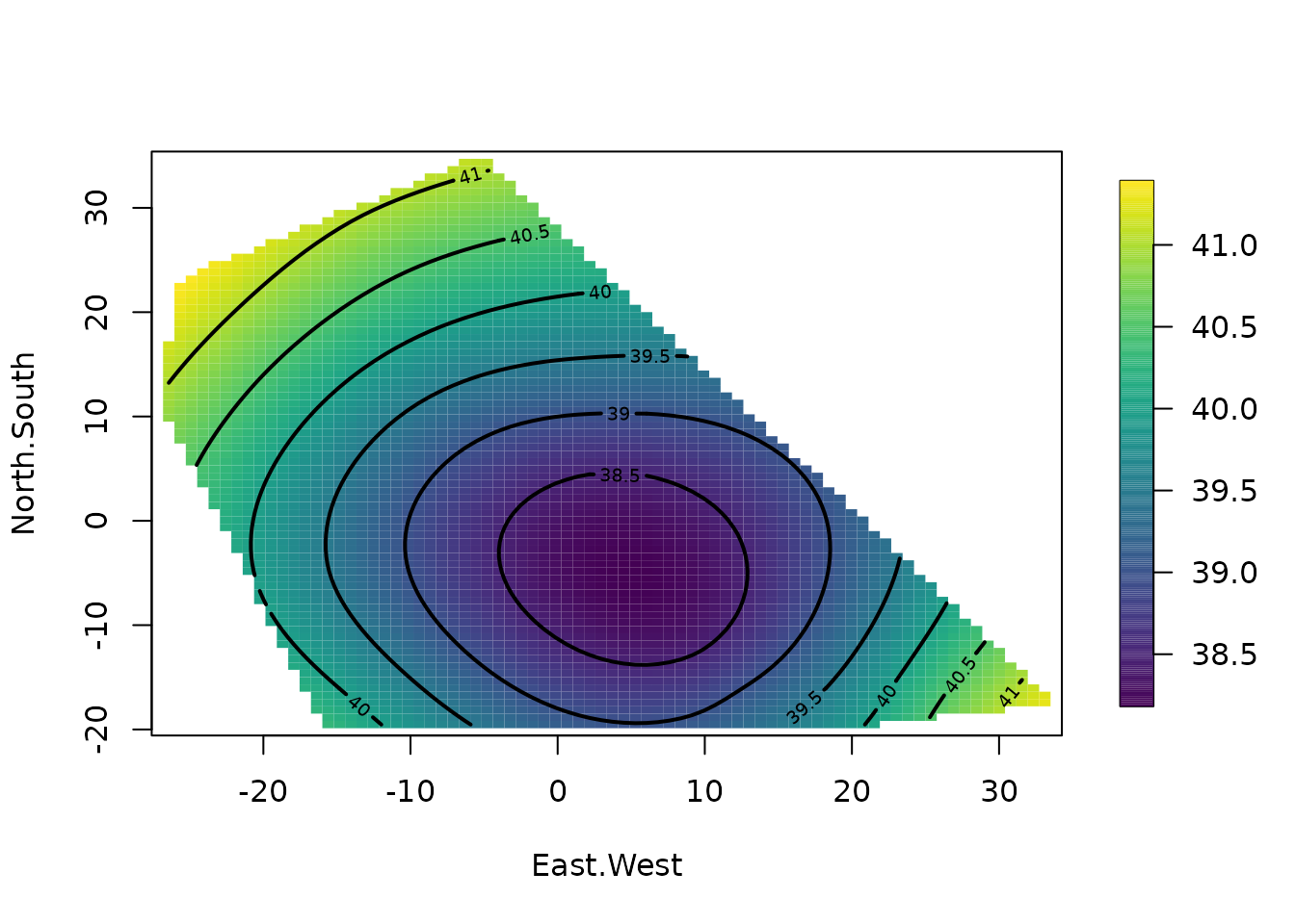
# NOTE: the predict function is quite flexible:
look <- predict(fit, lambda = 2.0)
#  evaluates the estimate at lambda =2.0  _not_ the GCV estimate
#  it does so very efficiently from the Krig fit object.

look <- predict(fit, df = 7.5)
#  evaluates the estimate at the lambda values such that
#  the effective degrees of freedom is 7.5
str(look)
#>  num [1:20, 1] 36.8 37.9 36.9 38.2 38.1 ...
compare this to fitting a thin plate spline with lambda chosen so that there are 7.5 effective degrees of freedom in estimate.
# Note that the GCV function is still computed and minimized
# but the lambda values used correpsonds to 7.5 df.
fit1 <- Tps(ChicagoO3$x, ChicagoO3$y, df = 7.5)

set.panel(2, 2)
#> plot window will lay out plots in a 2 by 2 matrix
plot(fit1) # four diagnostic plots of  fit and residuals.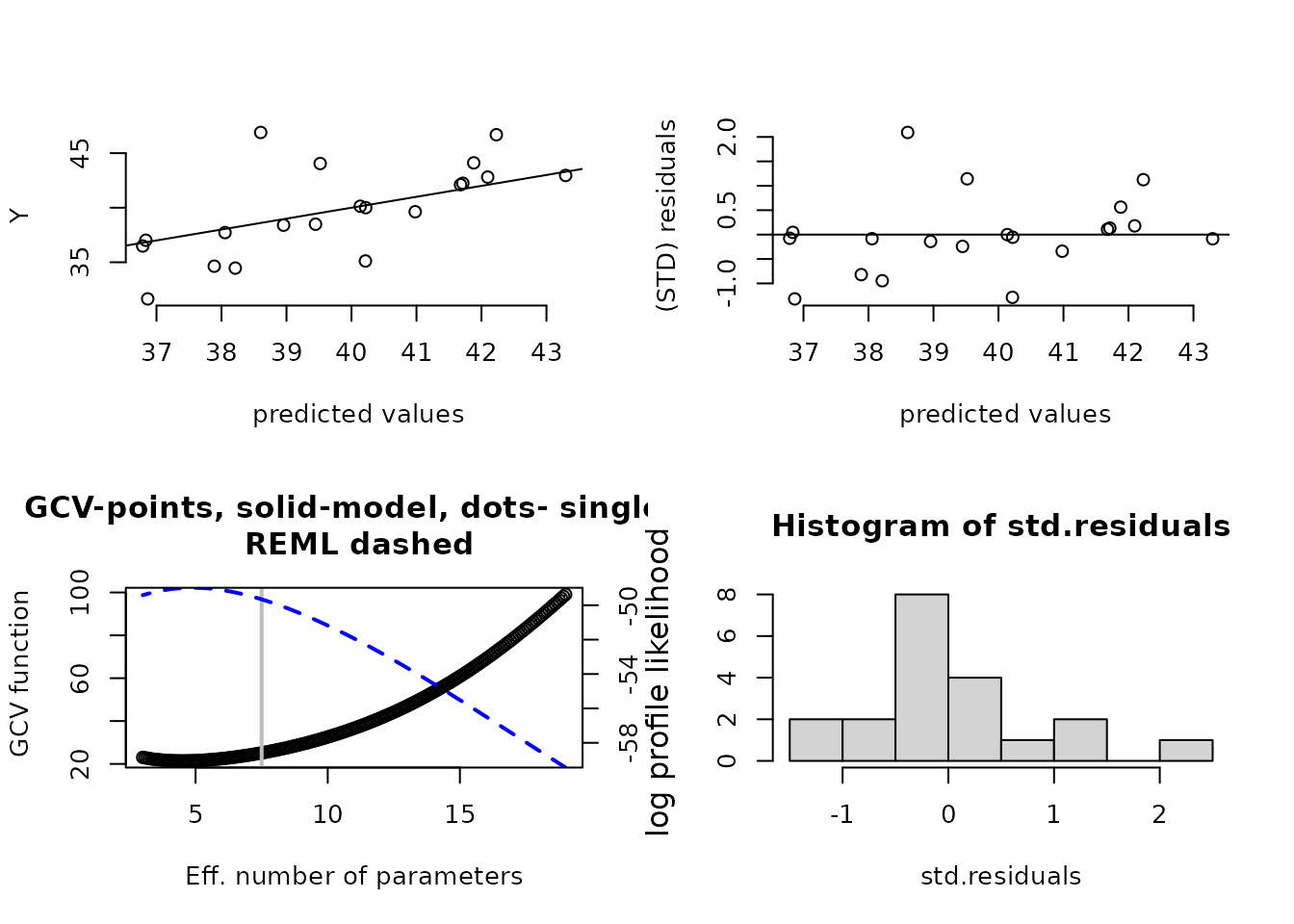
# GCV function (lower left) has vertical line at 7.5 df.
set.panel()
#> plot window will lay out plots in a 1 by 1 matrix

# The basic matrix decompositions are the same for
# both fit and fit1 objects.

# predict( fit1) is the same as predict( fit, df=7.5)
# predict( fit1, lambda= fit$lambda) is the same as predict(fit)
# predict onto a grid that matches the ranges of the data.
out.p <- predictSurface(fit)
image(out.p)
# the surface function (e.g. surface( fit)) essentially combines
# the two steps above

# predict at different effective number of parameters
out.p <- predictSurface(fit, df = 10)
1.2. Predicting average daily minimum temperature for spring in Colorado
Predicting on a grid along with a covariate. > 把高程Z作为协变量。
data(COmonthlyMet)
length(CO.tmin.MAM.climate)
#> [1] 376
# Ipaper::print2(CO.loc, CO.elev, CO.Grid, CO.elevGrid)

# # NOTE to create an 4km elevation grid:
# data(PRISMelevation);
# CO.elev1 <- crop.image(PRISMelevation, CO.loc)
# CO.Grid1<- CO.elev1[c("x","y")] # then use same grid for the predictions
obj <- Tps(CO.loc, CO.tmin.MAM.climate, Z = CO.elev)

# Note the size of `CO.Grid` and `CO.elevGrid` should be same.
out.p <- predictSurface(obj, CO.Grid, ZGrid = CO.elevGrid)
imagePlot(out.p)
US(add = TRUE, col = "grey")
contour(CO.elevGrid, add = TRUE, levels = c(2000), col = "black")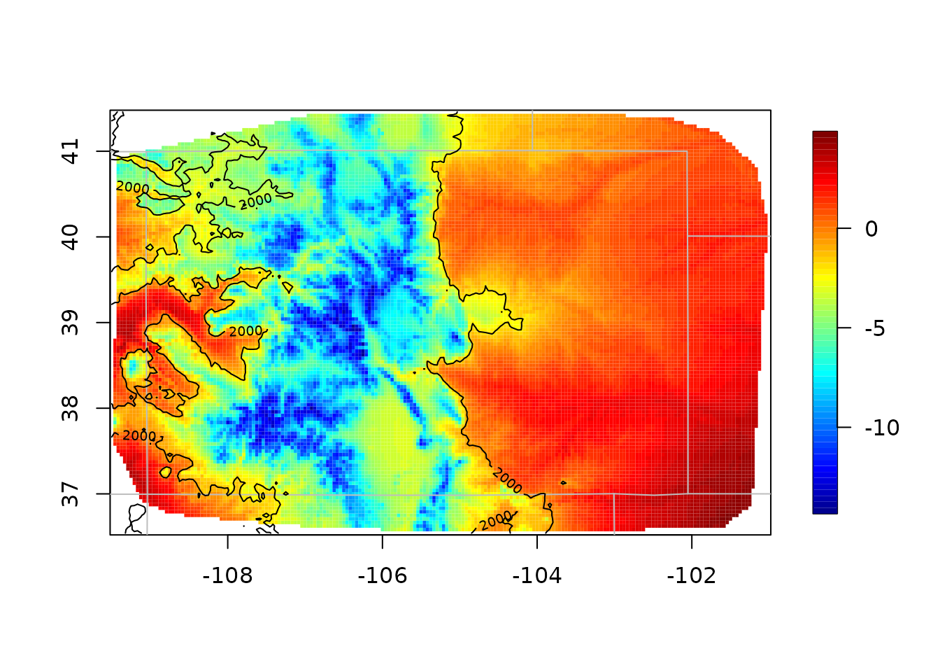
1.3. A 1-d example with confidence intervals
out <- Tps(rat.diet$t, rat.diet$trt) # lambda found by GCV
out
#> Call:
#> Tps(x = rat.diet$t, Y = rat.diet$trt)
#>
#>  Number of Observations:                39
#>  Number of parameters in the null space 2
#>  Parameters for fixed spatial drift     2
#>  Model degrees of freedom:              7.5
#>  Residual degrees of freedom:           31.5
#>  GCV estimate for tau:                  1.387
#>  MLE for tau:                           1.321
#>  MLE for sigma:                         4695
#>  lambda                                 0.00037
#>  User supplied sigma                    NA
#>  User supplied tau^2                    NA
#> Summary of estimates:
#>                  lambda      trA      GCV   tauHat -lnLike Prof converge
#> GCV        0.0003714897 7.460039 2.377626 1.386660     71.06878        2
#> GCV.model            NA       NA       NA       NA           NA       NA
#> GCV.one    0.0003714897 7.460039 2.377626 1.386660           NA        2
#> RMSE                 NA       NA       NA       NA           NA       NA
#> pure error           NA       NA       NA       NA           NA       NA
#> REML       0.0008674536 6.236239 2.404436 1.421252     70.76618        6

plot(out$x, out$y)
xgrid <- seq(min(out$x), max(out$x), , 100)
fhat <- predict(out, xgrid)
lines(xgrid, fhat, )
SE <- predictSE(out, xgrid)
lines(xgrid, fhat + 1.96 * SE, col = "red", lty = 2)
lines(xgrid, fhat - 1.96 * SE, col = "red", lty = 2)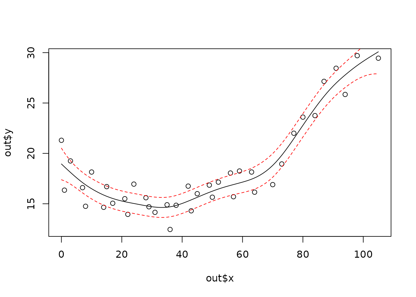
# compare to the (uch faster) B spline algorithm
#  sreg(rat.diet$t, rat.diet$trt)

# Here is a 1-d example with 95 percent  CIs  where sreg would not work:
#  sreg would give the right estimate here but not the right CI's
x <- seq(0, 1, , 8)
y <- sin(3 * x)
out <- Tps(x, y) # lambda found by GCV
#> Warning:
#> Grid searches over lambda (nugget and sill variances) with  minima at the endpoints:
#>   (GCV) Generalized Cross-Validation
#>    minimum at  right endpoint  lambda  =  1.701355e-05 (eff. df= 7.600005 )
plot(out$x, out$y)
xgrid <- seq(min(out$x), max(out$x), , 100)
fhat <- predict(out, xgrid)
lines(xgrid, fhat, lwd = 2)
SE <- predictSE(out, xgrid)
lines(xgrid, fhat + 1.96 * SE, col = "red", lty = 2)
lines(xgrid, fhat - 1.96 * SE, col = "red", lty = 2)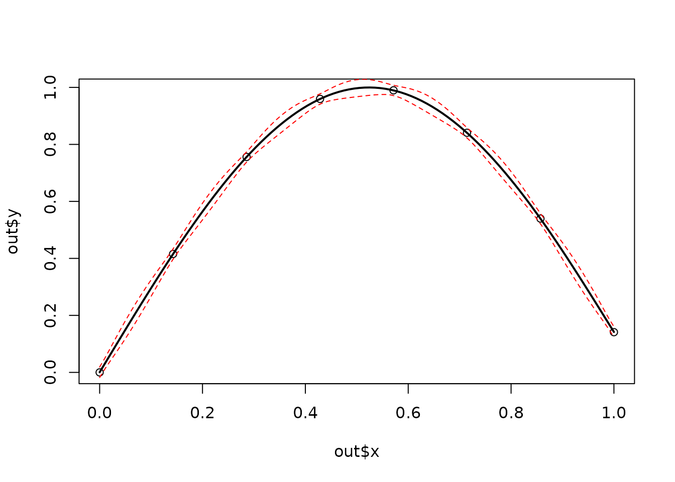
1.4. Add a covariate to the fixed part of model
set.panel(1, 3)
#> plot window will lay out plots in a 1 by 3 matrix
# without elevation covariate
out0 <- Tps(RMprecip$x, RMprecip$y)
surface(out0)
US(add = TRUE, col = "grey")

# with elevation covariate
out <- Tps(RMprecip$x, RMprecip$y, Z = RMprecip$elev)

# NOTE: out$d[4] is the estimated elevation coefficient
# it is easy to get the smooth surface separate from the elevation.
out.p <- predictSurface(out, drop.Z = TRUE)
surface(out.p)
US(add = TRUE, col = "grey")

# and if the estimate is of high resolution and you get by with
# a simple discretizing -- does not work in this case!
quilt.plot(out$x, out$fitted.values)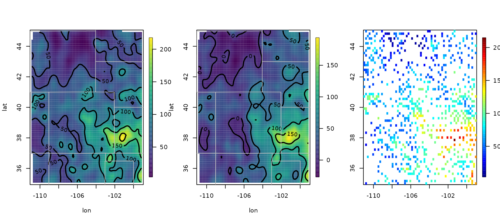
1.5. Third
把这个案例,改成
fastTps
# the exact way to do this is evaluate the estimate on a grid where you also have elevations
# An elevation DEM from the PRISM climate data product (4km resolution)
data(RMelevation)

grid.list <- list(x = RMelevation$x, y = RMelevation$y)

# Ipaper::print2(RMelevation, grid.list)

# this is the linear fixed part of the second spatial model:
# lon, lat and elevation
fit.full <- predictSurface(out, grid.list, ZGrid = RMelevation)

fit0 <- predictSurface(out0, grid.list) # without elevation

fit.fixed <- predictSurface(out, grid.list, just.fixed = TRUE, ZGrid = RMelevation) # lon, lat, elev

fit.smooth <- predictSurface(out, grid.list, drop.Z = TRUE) # smooth part + linear lon lat terms

set.panel(2, 2)
#> plot window will lay out plots in a 2 by 2 matrix

image.plot(fit0)
title("First spatial model (without elevation)")

image.plot(fit.fixed)
title("Fixed part: linear(lon, lat, elev)")

image.plot(fit.smooth)
title("Smooth part (smooth + linear(lon, lat))")

US(add = TRUE)
image.plot(fit.full)
title("Full prediction second model")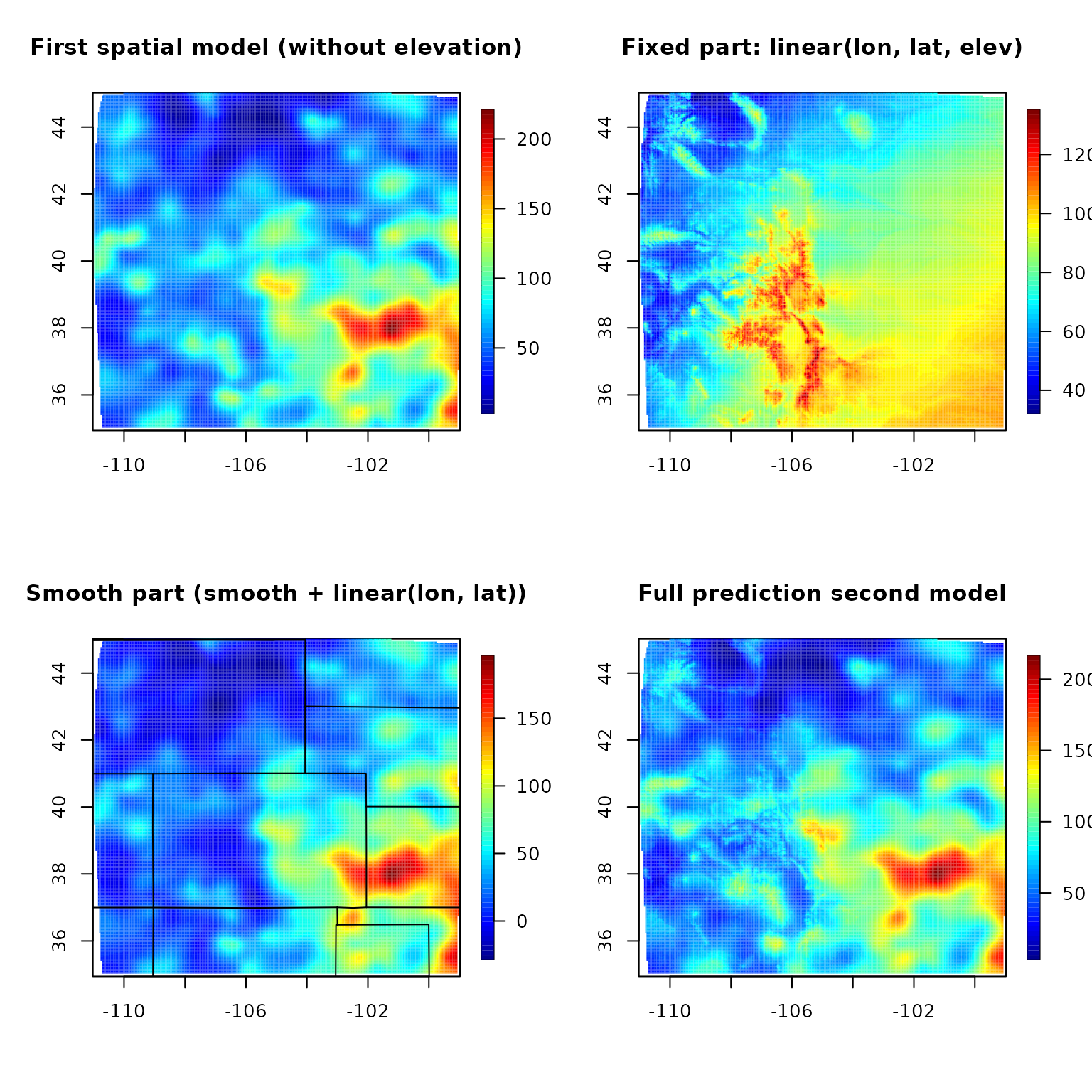
set.panel()
#> plot window will lay out plots in a 1 by 1 matrix
1.6. simulation reusing Tps/Krig object
str(rat.diet)
#> 'data.frame':    39 obs. of  3 variables:
#>  $ t  : num  0 1 3 7 8 10 14 15 17 21 ...
#>  $ con: num  20.5 19.4 22.2 17.9 19.9 ...
#>  $ trt: num  21.3 16.4 19.2 16.6 14.8 ...

fit <- Tps(rat.diet$t, rat.diet$trt)
true <- fit$fitted.values
N <- length(fit$y)
temp <- matrix(NA, ncol = 50, nrow = N)
tau <- fit$tauHat.GCV
for (k in 1:50) {
  ysim <- true + tau * rnorm(N)
  temp[, k] <- predict(fit, y = ysim)
}
matplot(fit$x, temp, type = "l")
2. Fast Tps
# Note: aRange = 3 degrees is a very generous taper range.
# Use some trial `aRange` value with `rdist.nearest` to determine a
# a useful taper. Some empirical studies suggest that in the
# interpolation case in 2 d the taper should be large enough to
# about 20 non zero nearest neighbors for every location.
# m = 2, p = 2m - d = 2
out2 <- fastTps(RMprecip$x, RMprecip$y,
m = 2, aRange = 3.0,
profileLambda = FALSE
)
# Note that fastTps produces a object of classes spatialProcess and mKrig
# so one can use all the overloaded functions that are defined for these classes.
# predict, predictSE, plot, sim.spatialProcess
#
# summary of what happened note estimate of effective degrees of freedom
# profiling on lambda has been turned off to make this run quickly
# but it is suggested that one examines the the profile likelihood over lambda
print(out2)
#> CALL:
#> fastTps(x = RMprecip$x, Y = RMprecip$y, m = 2, aRange = 3, profileLambda = FALSE)
#>
#> SUMMARY OF MODEL FIT:
#>
#> Number of Observations: 806
#> Degree of polynomial in fixed part: 1
#> Total number of parameters in fixed part: 3
#> sigma Process stan. dev: 22.53
#> tau Nugget stan. dev: 25.99
#> lambda tau^2/sigma^2: 1.33
#> aRange parameter (in units of distance): 3
#> Approx. degrees of freedom for curve 106.2
#> Standard Error of df estimate: 2.496
#> log Likelihood: -3871.12060412435
#> log Likelihood REML: -3879.17851011222
#>
#> ESTIMATED COEFFICIENTS FOR FIXED PART:
#>
#> estimate SE pValue
#> d1 756.400 106.5000 1.202e-12
#> d2 4.425 0.9369 2.317e-06
#> d3 -5.471 1.1070 7.698e-07
#>
#> COVARIANCE MODEL: wendland.cov
#> Non-default covariance arguments and their values
#> k :
#> [1] 2
#> Dist.args :
#> $method
#> [1] "euclidean"
#>
#> aRange :
#> [1] 3
#> Nonzero entries in covariance matrix 119816
#>
#> SUMMARY FROM Max. Likelihood ESTIMATION:
#> Parameters found from optim:
#> lambda
#> 1.330438
#> Approx. confidence intervals for MLE(s)
#> lower95% upper95%
#> lambda 0.9586872 1.846342
#>
#> Note: MLEs for tau and sigma found analytically from lambda
#>
#> Summary from estimation:
#> lnProfileLike.FULL lnProfileREML.FULL lnLike.FULL lnREML.FULL
#> -3871.120604 -3879.178510 NA NA
#> lambda tau sigma2 aRange
#> 1.330438 25.991494 507.771046 3.000000
#> eff.df GCV
#> 106.205992 775.347011
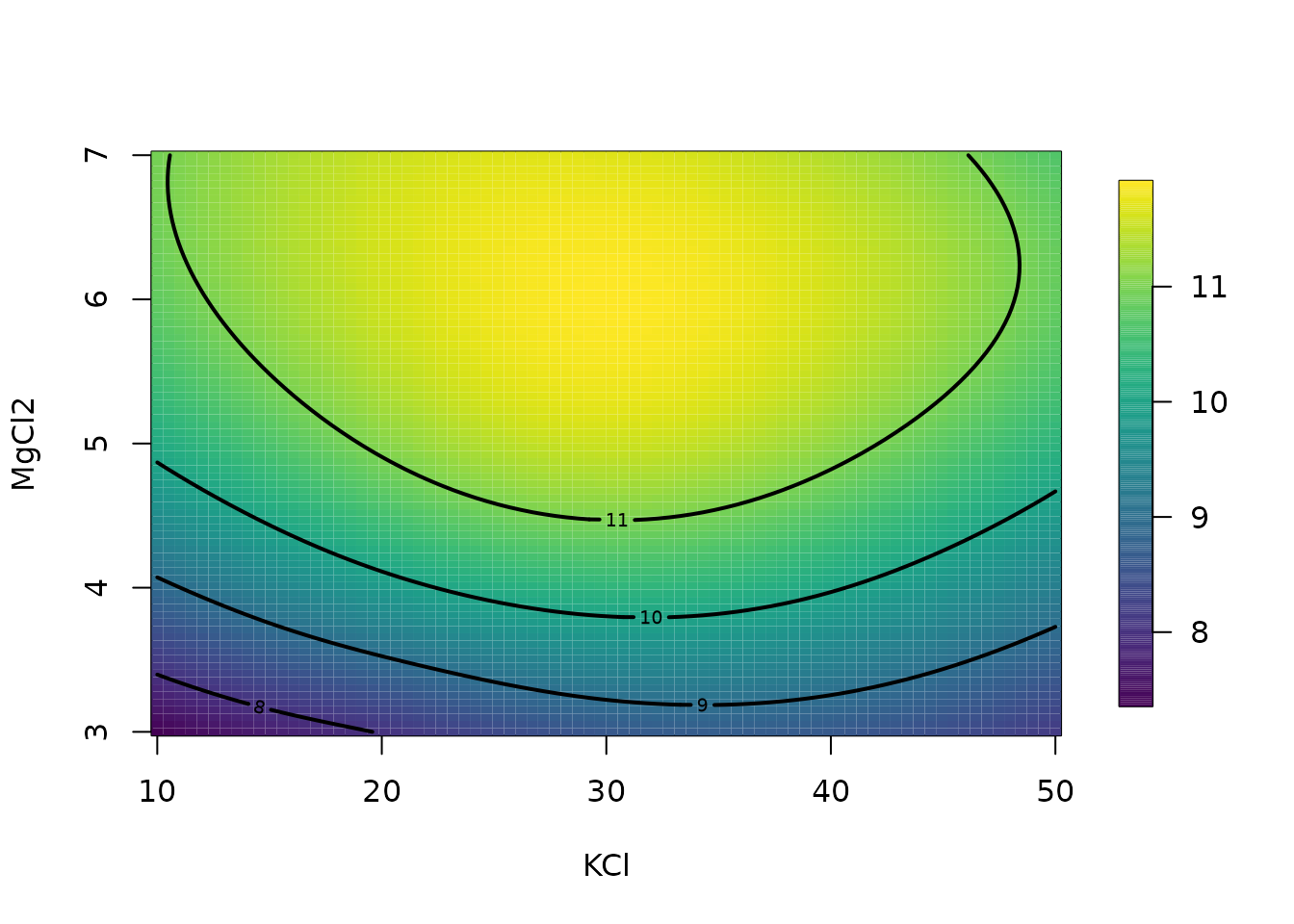
set.panel(1, 2)
#> plot window will lay out plots in a 1 by 2 matrix
surface(out2)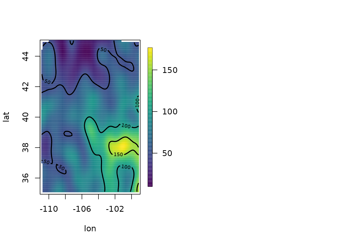
Now use great circle distance for this smooth.
Here “aRange” for the taper support is the great circle distance in degrees latitude. Typically for data analysis it more convenient to think in degrees. A degree of latitude is about 68 miles (111 km).
fastTps(RMprecip$x, RMprecip$y, m = 2, lon.lat = TRUE, aRange = 210) -> out3
print(out3) # note the effective degrees of freedom is different.
#> CALL:
#> fastTps(x = RMprecip$x, Y = RMprecip$y, m = 2, aRange = 210,
#>     lon.lat = TRUE)
#>
#>  SUMMARY OF MODEL FIT:
#>
#>  Number of Observations:                    806
#>  Degree of polynomial in fixed part:        1
#>  Total number of parameters in fixed part:  3
#>  sigma Process stan. dev:                   23.38
#>  tau  Nugget stan. dev:                     26.25
#>  lambda   tau^2/sigma^2:                    1.26
#>  aRange parameter (in units of distance):   210
#>  Approx.  degrees of freedom for curve      91.64
#>     Standard Error of df estimate:          2.344
#>  log Likelihood:                            -3869.75983890003
#>  log Likelihood REML:                       -3877.51050412707
#>
#>  ESTIMATED COEFFICIENTS FOR FIXED PART:
#>
#>    estimate      SE    pValue
#> d1  772.400 120.600 1.530e-10
#> d2    4.590   1.058 1.431e-05
#> d3   -5.431   1.279 2.182e-05
#>
#>  COVARIANCE MODEL: wendland.cov
#>    Non-default covariance arguments and their values
#> k :
#> [1] 2
#> Dist.args :
#> $method
#> [1] "greatcircle"
#>
#> aRange :
#> [1] 210
#> Nonzero entries in covariance matrix  152398
#>
#> SUMMARY FROM Max. Likelihood ESTIMATION:
#> Parameters found from optim:
#>   lambda
#> 1.260473
#> Approx. confidence intervals for MLE(s)
#>         lower95% upper95%
#> lambda 0.8798356 1.805784
#>
#>  Note: MLEs for  tau and sigma found analytically from lambda
#>
#> Summary from estimation:
#> lnProfileLike.FULL lnProfileREML.FULL        lnLike.FULL        lnREML.FULL
#>       -3869.759839       -3877.510504                 NA                 NA
#>             lambda                tau             sigma2             aRange
#>           1.260473          26.247003         546.544737         210.000000
#>             eff.df                GCV
#>          91.642338         774.862042
surface(out3)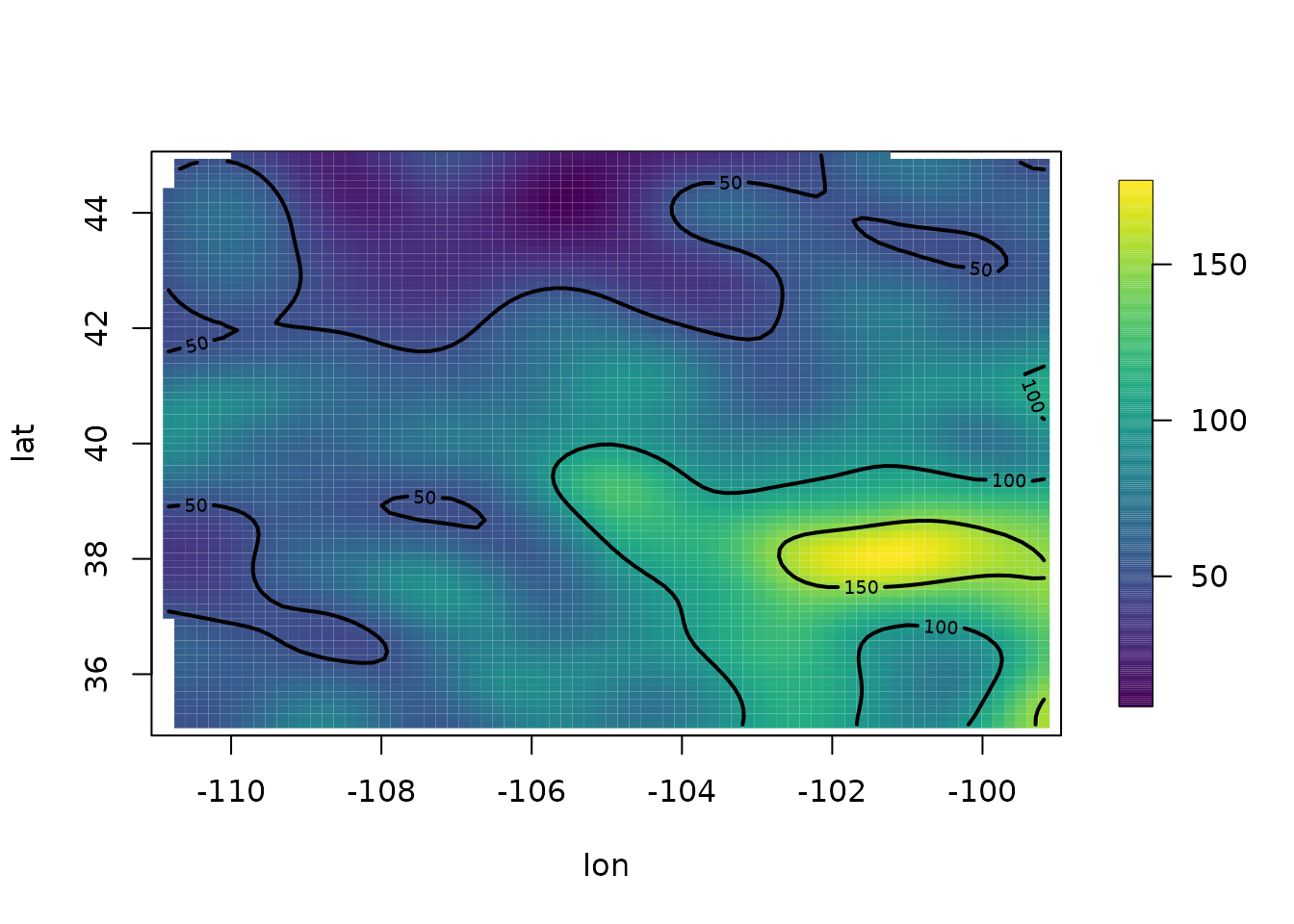
set.panel()
#> plot window will lay out plots in a 1 by 1 matrix