fastTps

1. Tps

library(fields)
#> Loading required package: spam
#> Spam version 2.9-1 (2022-08-07) is loaded.
#> Type 'help( Spam)' or 'demo( spam)' for a short introduction 
#> and overview of this package.
#> Help for individual functions is also obtained by adding the
#> suffix '.spam' to the function name, e.g. 'help( chol.spam)'.
#> 
#> Attaching package: 'spam'
#> The following objects are masked from 'package:base':
#> 
#>     backsolve, forwardsolve
#> Loading required package: viridis
#> Loading required package: viridisLite
#> 
#> Try help(fields) to get started.

# An elevation DEM from the PRISM climate data product (4km resolution)
data(RMelevation)
grid.list <- RMelevation[1:2]

# Ipaper::print2(RMelevation, grid.list)
str(RMprecip)
#> List of 3
#>  $ x   :'data.frame':    806 obs. of  2 variables:
#>   ..$ lon: num [1:806] -111 -110 -110 -109 -110 ...
#>   ..$ lat: num [1:806] 36.7 36.1 35.7 36.4 37 ...
#>  $ elev: num [1:806] 2196 1710 1937 1976 1696 ...
#>  $ y   : num [1:806] 81 63 36 46 33 40 97 99 58 32 ...

1.1. Add a covariate to the fixed part of model

out0 <- Tps(RMprecip$x, RMprecip$y) # without elevation covariate
out  <- Tps(RMprecip$x, RMprecip$y, Z = RMprecip$elev) # with elevation covariate

# NOTE: out$d[4] is the estimated elevation coefficient
# it is easy to get the smooth surface separate from the elevation.
out.p <- predictSurface(out, drop.Z = TRUE)

set.panel(2, 2)
#> plot window will lay out plots in a 2 by 2 matrix
surface(out0)
US(add = TRUE, col = "grey")

surface(out.p) # delete elev
US(add = TRUE, col = "grey")

# and if the estimate is of high resolution and you get by with
# a simple discretizing -- does not work in this case!
quilt.plot(out$x, out$fitted.values)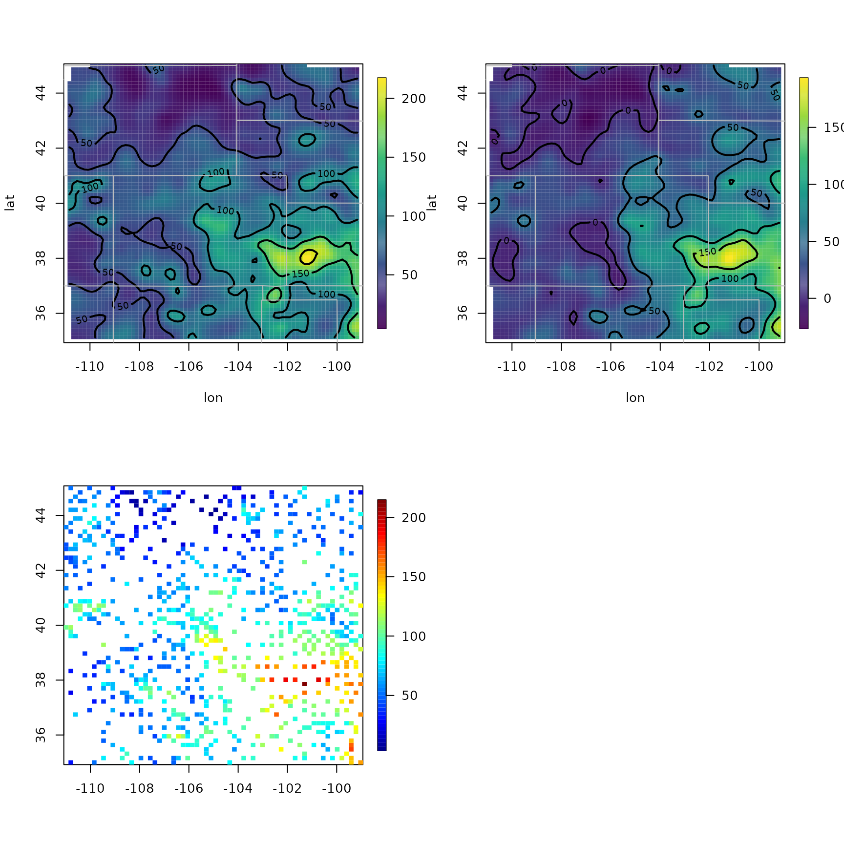

1.2. 分解各个组分

fit.full <- predictSurface(out, grid.list, ZGrid = RMelevation)

fit0 <- predictSurface(out0, grid.list) # without elevation

fit.fixed <- predictSurface(out, grid.list, just.fixed = TRUE, ZGrid = RMelevation) # lon, lat, elev

fit.smooth <- predictSurface(out, grid.list, drop.Z = TRUE) # smooth part + linear lon lat terms

set.panel(2, 2)
#> plot window will lay out plots in a 2 by 2 matrix

image.plot(fit0)
title("First spatial model (without elevation)")

image.plot(fit.fixed)
title("Fixed part: linear(lon, lat, elev)")

image.plot(fit.smooth)
title("Smooth part (smooth + linear(lon, lat))")

US(add = TRUE)
image.plot(fit.full)
title("Full prediction second model")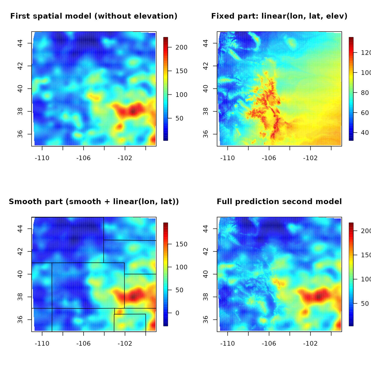

set.panel()
#> plot window will lay out plots in a 1 by 1 matrix

2. fastTps

system.time({
  r_low <- Tps(RMprecip$x, RMprecip$y, Z = RMprecip$elev) # with elevation covariate
})
#>    user  system elapsed 
#>   0.468   0.075   0.304

# not always work
system.time({
  r_fst1 <- fastTps(RMprecip$x, RMprecip$y, Z = RMprecip$elev, 
    aRange = 200, lon.lat = TRUE) # with elevation covariate
})
#>    user  system elapsed 
#>   2.368   0.651   1.587

system.time({
  r_fst2 <- fastTps(RMprecip$x, RMprecip$y,
    # m = 2, 
    aRange = 3.0,
    profileLambda = FALSE
  )
})
#>    user  system elapsed 
#>   2.629   0.838   1.768
# in this case not work