Example01
# df = data.table(chicagoNMMAPS)
head(chicagoNMMAPS, 3)
#>         date time year month doy      dow death cvd resp       temp   dptp
#> 1 1987-01-01    1 1987     1   1 Thursday   130  65   13 -0.2777778 31.500
#> 2 1987-01-02    2 1987     1   2   Friday   150  73   14  0.5555556 29.875
#> 3 1987-01-03    3 1987     1   3 Saturday   101  43   11  0.5555556 27.375
#>    rhum     pm10       o3
#> 1 95.50 26.95607 4.376079
#> 2 88.25       NA 4.929803
#> 3 89.50 32.83869 3.751079

cb1.pm <- crossbasis(chicagoNMMAPS$pm10, lag = 15,
  argvar = list(fun = "lin"),
  arglag = list(fun = "poly", degree = 4)
)

cb1.temp <- crossbasis(chicagoNMMAPS$temp, lag = 3,
  argvar = list(df = 5), # ns
  arglag = list(fun = "strata", breaks = 1)
)
summary(cb1.pm)
#> CROSSBASIS FUNCTIONS
#> observations: 5114
#> range: -3.049835 to 356.1768
#> lag period: 0 15
#> total df:  5
#>
#> BASIS FOR VAR:
#> fun: lin
#> intercept: FALSE
#>
#> BASIS FOR LAG:
#> fun: poly
#> degree: 4
#> scale: 15
#> intercept: TRUE
str(cb1.temp)
#>  'crossbasis' num [1:5114, 1:10] NA NA NA 2.01 2.03 ...
#>  - attr(*, "dimnames")=List of 2
#>   ..$ : NULL
#>   ..$ : chr [1:10] "v1.l1" "v1.l2" "v2.l1" "v2.l2" ...
#>  - attr(*, "df")= int [1:2] 5 2
#>  - attr(*, "range")= num [1:2] -26.7 33.3
#>  - attr(*, "lag")= num [1:2] 0 3
#>  - attr(*, "argvar")=List of 4
#>   ..$ fun           : chr "ns"
#>   ..$ knots         : num [1:4] 0.278 6.667 14.444 20.944
#>   ..$ intercept     : logi FALSE
#>   ..$ Boundary.knots: num [1:2] -26.7 33.3
#>  - attr(*, "arglag")=List of 5
#>   ..$ fun      : chr "strata"
#>   ..$ df       : int 2
#>   ..$ breaks   : num 1
#>   ..$ ref      : num 1
#>   ..$ intercept: logi TRUE
#>  - attr(*, "basisvar")= 'onebasis' num [1:5114, 1:5] 0.498 0.546 0.546 0.423 0.514 ...
#>   ..- attr(*, "fun")= chr "ns"
#>   ..- attr(*, "dimnames")=List of 2
#>   .. ..$ : NULL
#>   .. ..$ : chr [1:5] "b1" "b2" "b3" "b4" ...
#>   ..- attr(*, "degree")= int 3
#>   ..- attr(*, "knots")= num [1:4] 0.278 6.667 14.444 20.944
#>   ..- attr(*, "Boundary.knots")= num [1:2] -26.7 33.3
#>   ..- attr(*, "intercept")= logi FALSE
#>   ..- attr(*, "range")= num [1:2] -26.7 33.3
#>  - attr(*, "basislag")= 'onebasis' num [1:4, 1:2] 1 1 1 1 0 1 1 1
#>   ..- attr(*, "fun")= chr "strata"
#>   ..- attr(*, "dimnames")=List of 2
#>   .. ..$ : NULL
#>   .. ..$ : chr [1:2] "b1" "b2"
#>   ..- attr(*, "df")= int 2
#>   ..- attr(*, "breaks")= num 1
#>   ..- attr(*, "ref")= num 1
#>   ..- attr(*, "intercept")= logi TRUE
#>   ..- attr(*, "range")= num [1:2] 0 3
library(splines)
model1 <- glm(death ~ cb1.pm + cb1.temp + ns(time, 7 * 14) + dow,
family = quasipoisson(), chicagoNMMAPS
)
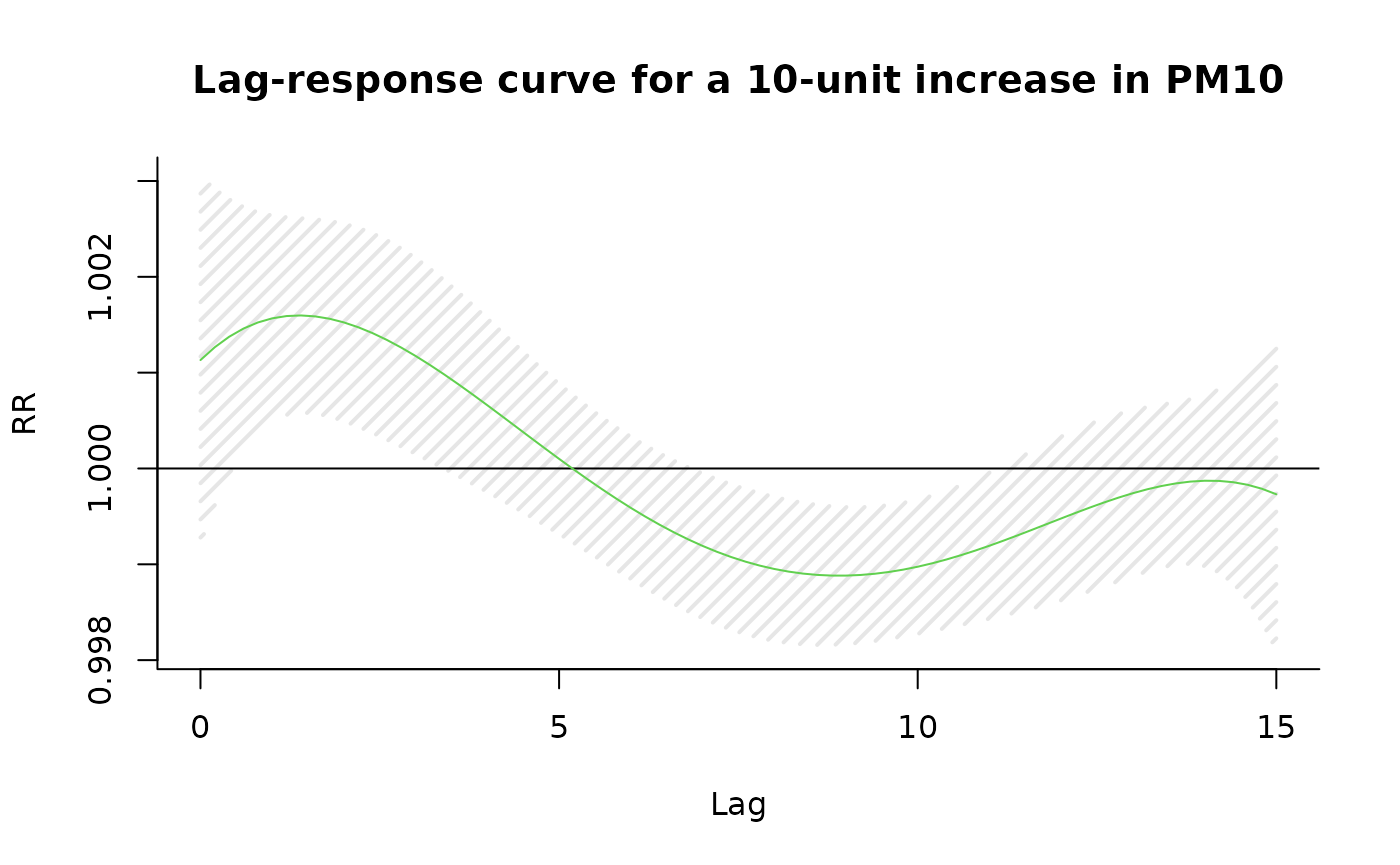
pred1.pm <- crosspred(cb1.pm, model1, at = 0:20, bylag = 0.2, cumul = TRUE)
plot(pred1.pm, "slices",
var = 10, col = 3, ylab = "RR", ci.arg = list(density = 15, lwd = 2),
main = "Lag-response curve for a 10-unit increase in PM10"
)
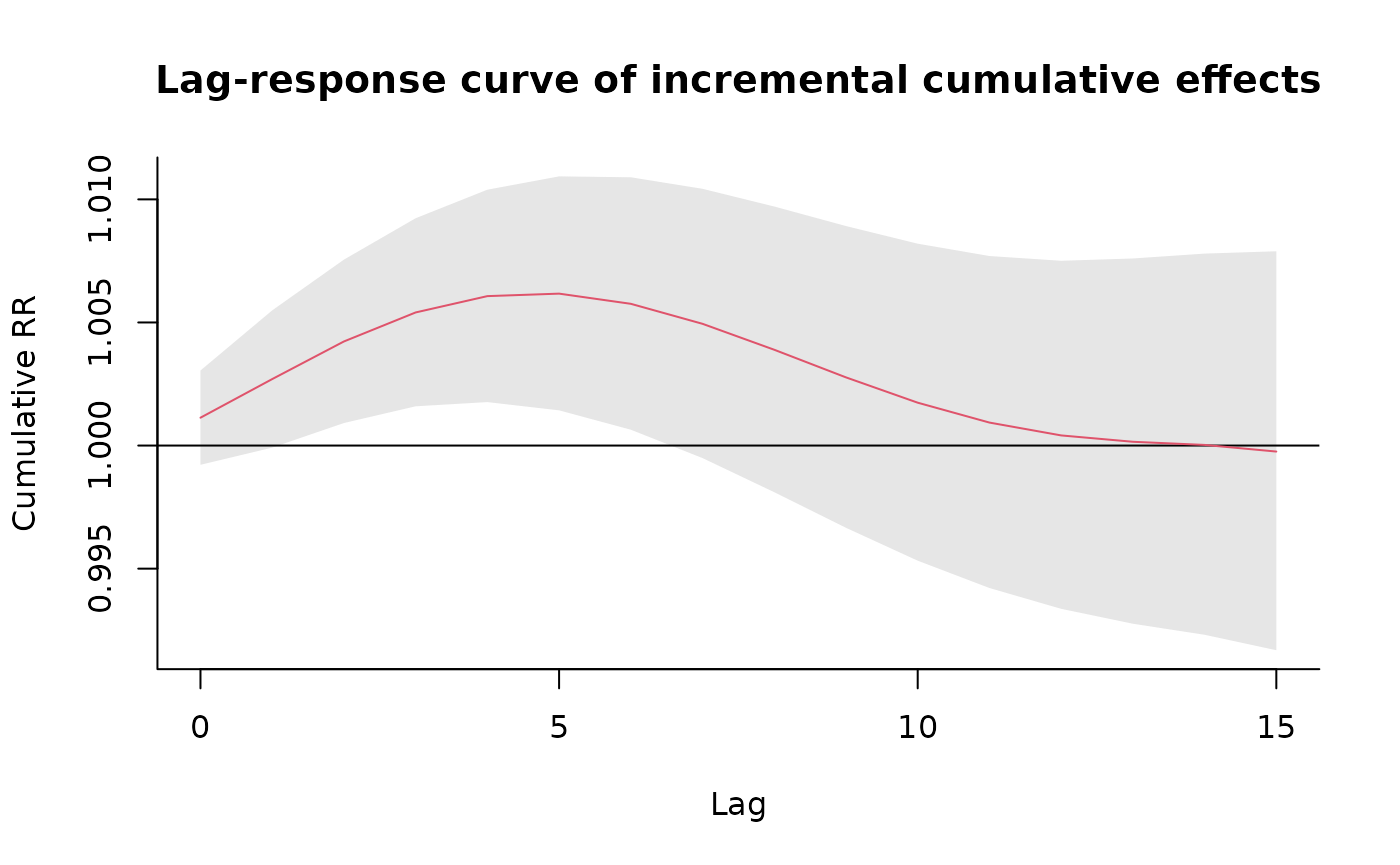
plot(pred1.pm, "slices",
  var = 10, col = 2, cumul = TRUE, ylab = "Cumulative RR",
  main = "Lag-response curve of incremental cumulative effects"
)
### code chunk number 9: example1slicesnoeval (eval = FALSE)

## plot(pred1.pm, "slices", var=10, col=3, ylab="RR", ci.arg=list(density=15,lwd=2),
##   main="Association with a 10-unit increase in PM10")
## plot(pred1.pm, "slices", var=10, col=2, cumul=TRUE, ylab="Cumulative RR",
##   main="Cumulative association with a 10-unit increase in PM10")
pred1.pm$allRRfit["10"]
#>        10
#> 0.9997563
cbind(pred1.pm$allRRlow, pred1.pm$allRRhigh)["10", ]
#> [1] 0.9916871 1.0078911

### code chunk number 11: dataseason
chicagoNMMAPSseas <- subset(chicagoNMMAPS, month %in% 6:9)
Example02
cb2.o3 <- crossbasis(chicagoNMMAPSseas$o3, lag = 5,
argvar = list(fun = "thr", thr = 40.3),
arglag = list(fun = "integer"),
group = chicagoNMMAPSseas$year
)
cb2.temp <- crossbasis(chicagoNMMAPSseas$temp, lag = 10,
argvar = list(fun = "thr", thr = c(15, 25)),
arglag = list(fun = "strata", breaks = c(2, 6)),
group = chicagoNMMAPSseas$year
)
### code chunk number 13: example2modelpred
model2 <- glm(death ~ cb2.o3 + cb2.temp + ns(doy, 4) + ns(time, 3) + dow,
family = quasipoisson(), chicagoNMMAPSseas
)
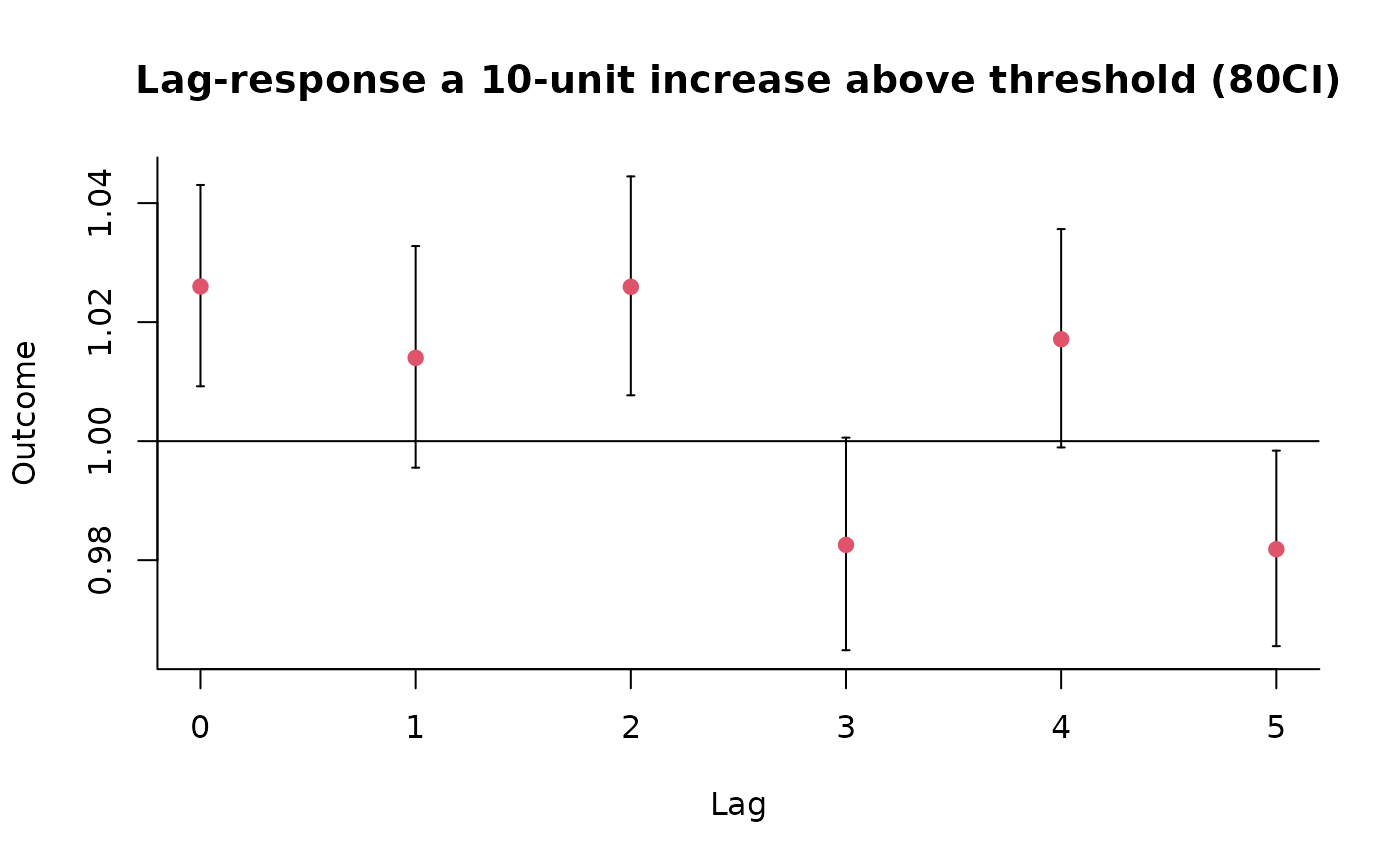
pred2.o3 <- crosspred(cb2.o3, model2, at = c(0:65, 40.3, 50.3))
### code chunk number 14: example2slices
plot(pred2.o3, "slices",
var = 50.3, ci = "bars", type = "p", col = 2, pch = 19,
ci.level = 0.80, main = "Lag-response a 10-unit increase above threshold (80CI)"
)
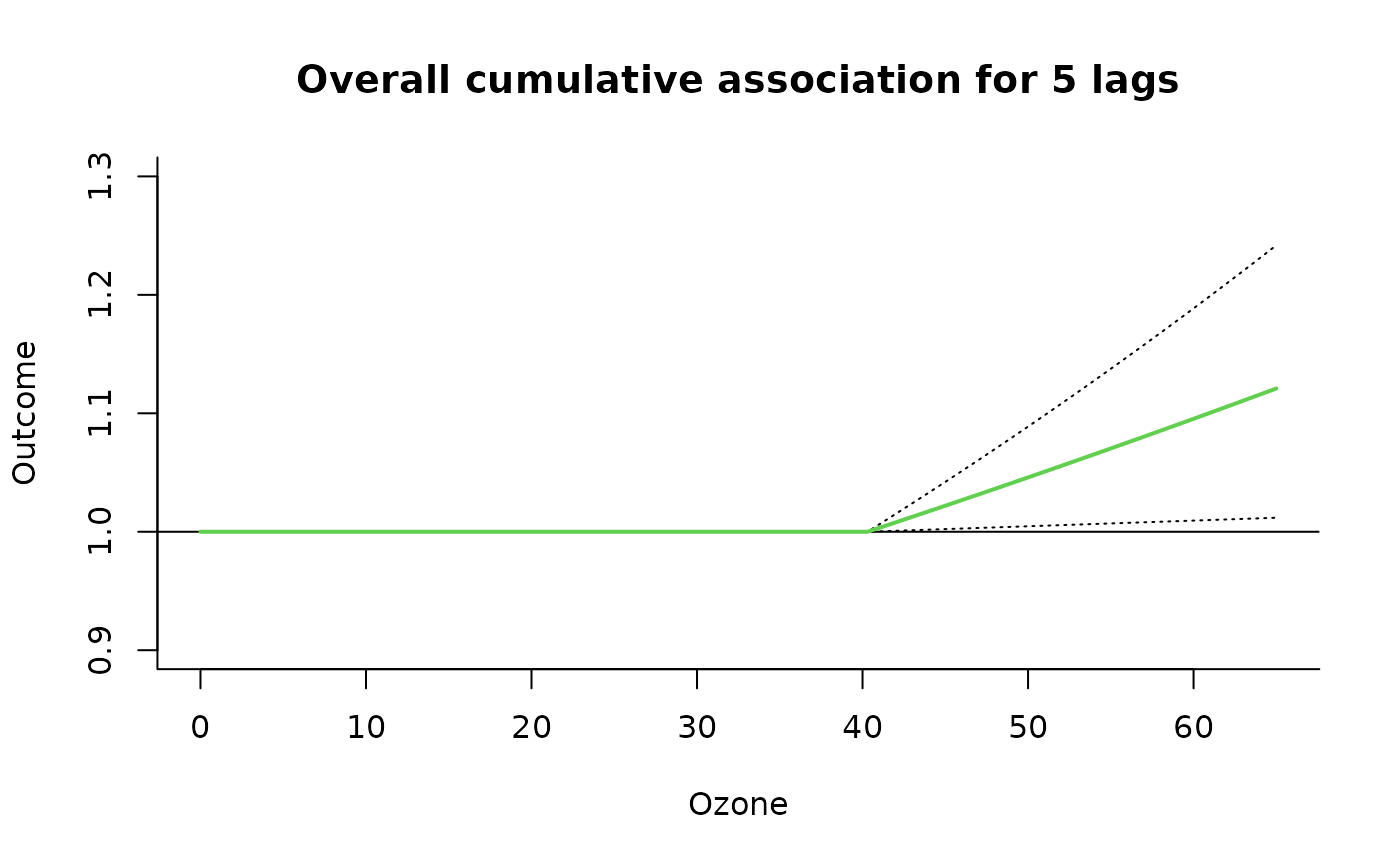
### code chunk number 15: example2overall
plot(pred2.o3, "overall",
  xlab = "Ozone", ci = "l", col = 3, ylim = c(0.9, 1.3), lwd = 2,
  ci.arg = list(col = 1, lty = 3), main = "Overall cumulative association for 5 lags"
)
### code chunk number 16: example2noeval1 (eval = FALSE)

## plot(pred2.o3, "slices", var=50.3, ci="bars", type="p", col=2, pch=19,
##   ci.level=0.80, main="Lag-response a 10-unit increase above threshold (80CI)")
## plot(pred2.o3,"overall",xlab="Ozone", ci="l", col=3, ylim=c(0.9,1.3), lwd=2,
##   ci.arg=list(col=1,lty=3), main="Overall cumulative association for 5 lags")

### code chunk number 17: example2effect
pred2.o3$allRRfit["50.3"]
#>     50.3
#> 1.047313
cbind(pred2.o3$allRRlow, pred2.o3$allRRhigh)["50.3", ]
#> [1] 1.004775 1.091652
Example03
cb3.pm <- crossbasis(chicagoNMMAPS$pm10, lag = 1,
argvar = list(fun = "lin"),
arglag = list(fun = "strata")
)
varknots <- equalknots(chicagoNMMAPS$temp, fun = "bs", df = 5, degree = 2)
lagknots <- logknots(30, 3)
cb3.temp <- crossbasis(chicagoNMMAPS$temp, lag = 30, argvar = list(
fun = "bs",
knots = varknots
), arglag = list(knots = lagknots))
### code chunk number 19: example3noeval (eval = FALSE)
## model3 <- glm(death ~ cb3.pm + cb3.temp + ns(time, 7*14) + dow,
## family=quasipoisson(), chicagoNMMAPS)
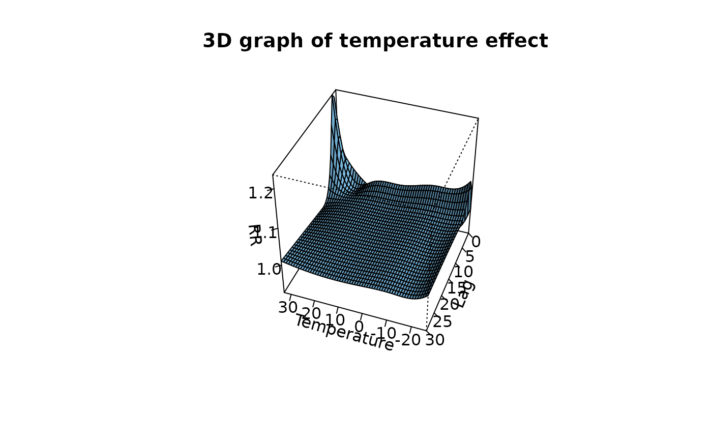
## pred3.temp <- crosspred(cb3.temp, model3, cen=21, by=1)
## plot(pred3.temp, xlab="Temperature", zlab="RR", theta=200, phi=40, lphi=30,
## main="3D graph of temperature effect")
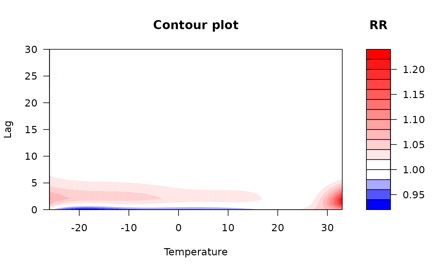
## plot(pred3.temp, "contour", xlab="Temperature", key.title=title("RR"),
## plot.title=title("Contour plot",xlab="Temperature",ylab="Lag"))
### code chunk number 20: example3plot3d
model3 <- glm(death ~ cb3.pm + cb3.temp + ns(time, 7 * 14) + dow,
family = quasipoisson(), chicagoNMMAPS
)
pred3.temp <- crosspred(cb3.temp, model3, cen = 21, by = 1)
plot(pred3.temp,
xlab = "Temperature", zlab = "RR", theta = 200, phi = 40, lphi = 30,
main = "3D graph of temperature effect"
)
### code chunk number 21: example3plotcontour
plot(pred3.temp, "contour",
  xlab = "Temperature", key.title = title("RR"),
  plot.title = title("Contour plot", xlab = "Temperature", ylab = "Lag")
)
### code chunk number 22: example3noeval2 (eval = FALSE)
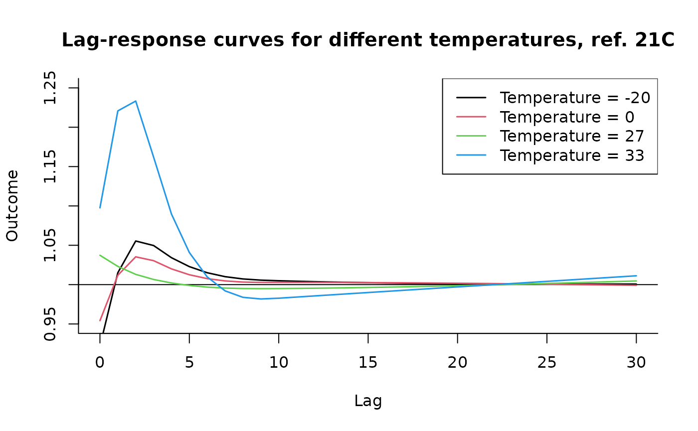
## plot(pred3.temp, "slices", var=-20, ci="n", col=1, ylim=c(0.95,1.25), lwd=1.5,
## main="Lag-response curves for different temperatures, ref. 21C")
## for(i in 1:3) lines(pred3.temp, "slices", var=c(0,27,33)[i], col=i+1, lwd=1.5)
## legend("topright",paste("Temperature =",c(-20,0,27,33)), col=1:4, lwd=1.5)
## plot(pred3.temp, "slices", var=c(-20,33), lag=c(0,5), col=4,
## ci.arg=list(density=40,col=grey(0.7)))
### code chunk number 23: example3slices
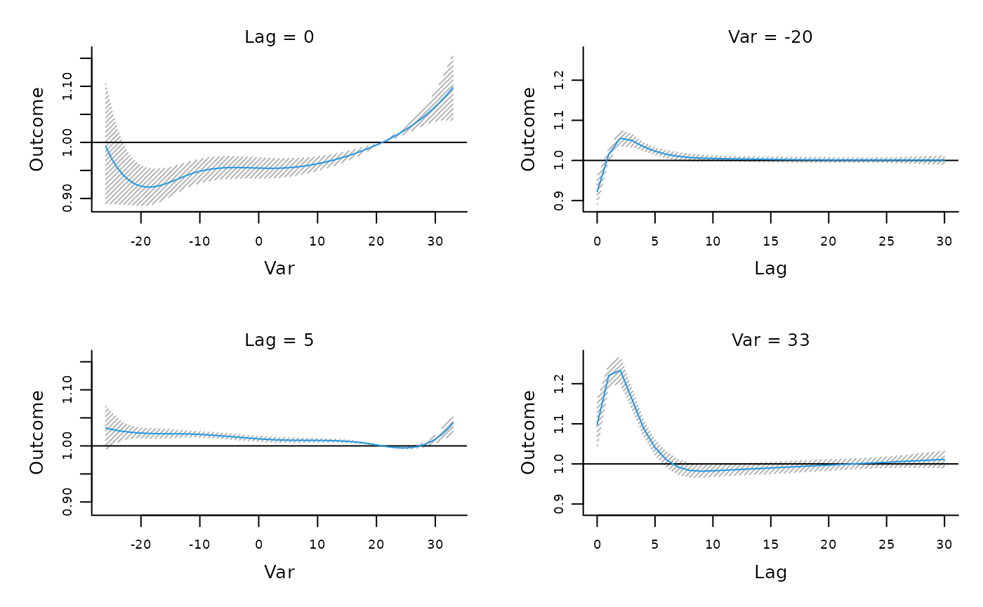
plot(pred3.temp, "slices",
var = -20, ci = "n", col = 1, ylim = c(0.95, 1.25), lwd = 1.5,
main = "Lag-response curves for different temperatures, ref. 21C"
)
for (i in 1:3) lines(pred3.temp, "slices", var = c(0, 27, 33)[i], col = i + 1, lwd = 1.5)
legend("topright", paste("Temperature =", c(-20, 0, 27, 33)), col = 1:4, lwd = 1.5)
### code chunk number 24: example3slices2

plot(pred3.temp, "slices",
  var = c(-20, 33), lag = c(0, 5), col = 4,
  ci.arg = list(density = 40, col = grey(0.7))
)
Example04
cb4 <- crossbasis(chicagoNMMAPS$temp, lag = 30,
argvar = list(fun = "thr", thr = c(10, 25)),
arglag = list(knots = lagknots)
)
model4 <- glm(death ~ cb4 + ns(time, 7 * 14) + dow,
family = quasipoisson(), chicagoNMMAPS
)
pred4 <- crosspred(cb4, model4, by = 1)
### code chunk number 26: example4reduce
redall <- crossreduce(cb4, model4)
redlag <- crossreduce(cb4, model4, type = "lag", value = 5)
redvar <- crossreduce(cb4, model4, type = "var", value = 33)
### code chunk number 27: example4dim
length(coef(pred4))
#> [1] 10
length(coef(redall))
#> [1] 2
length(coef(redlag))
#> [1] 2
length(coef(redvar))
#> [1] 5
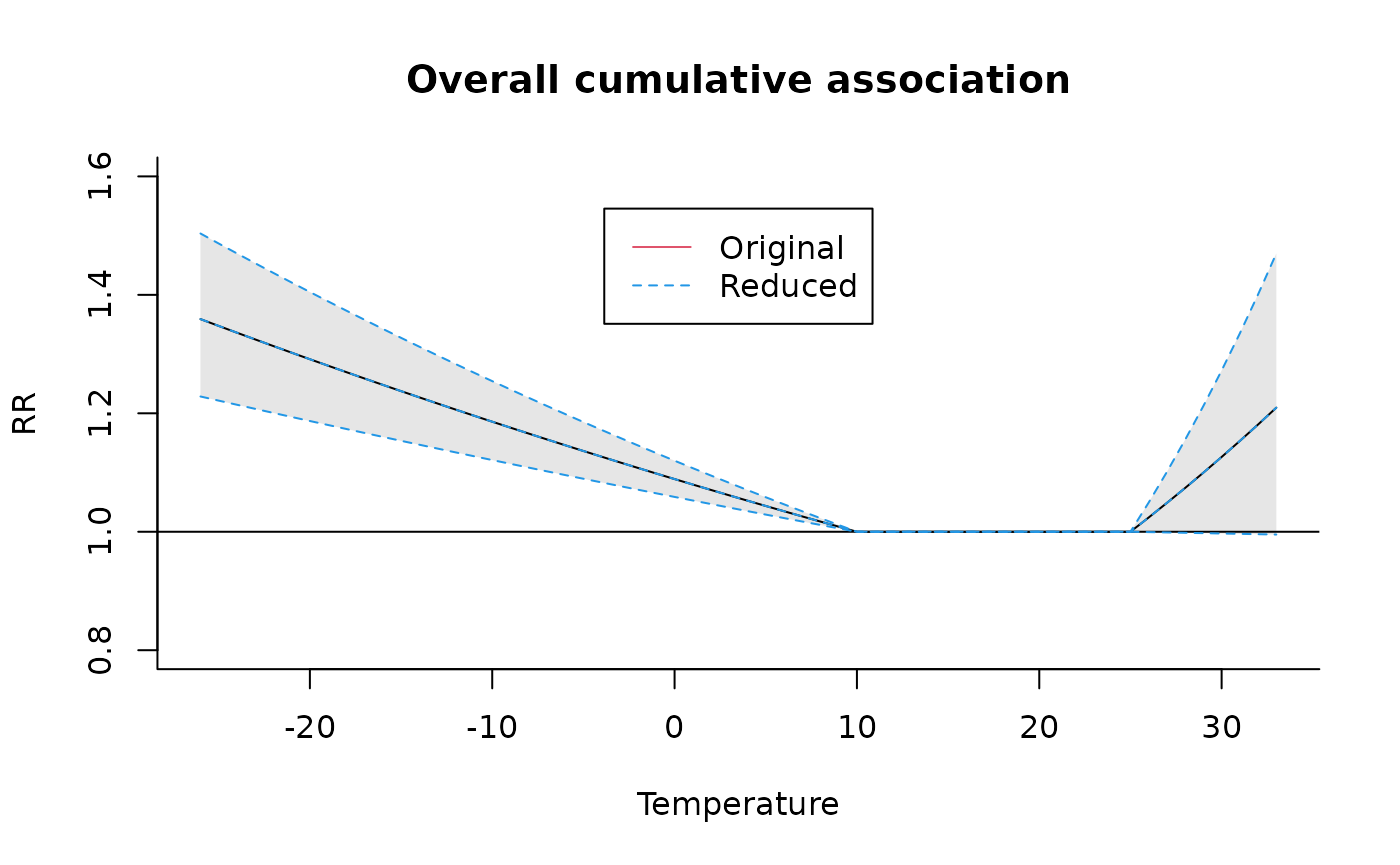
### code chunk number 28: example4plotall
plot(pred4, "overall",
xlab = "Temperature", ylab = "RR",
ylim = c(0.8, 1.6), main = "Overall cumulative association"
)
lines(redall, ci = "lines", col = 4, lty = 2)
legend("top", c("Original", "Reduced"), col = c(2, 4), lty = 1:2, ins = 0.1)
### code chunk number 29: example4reconstr
b4 <- onebasis(0:30, knots = attributes(cb4)$arglag$knots, intercept = TRUE)
pred4b <- crosspred(b4, coef = coef(redvar), vcov = vcov(redvar), model.link = "log", by = 1)
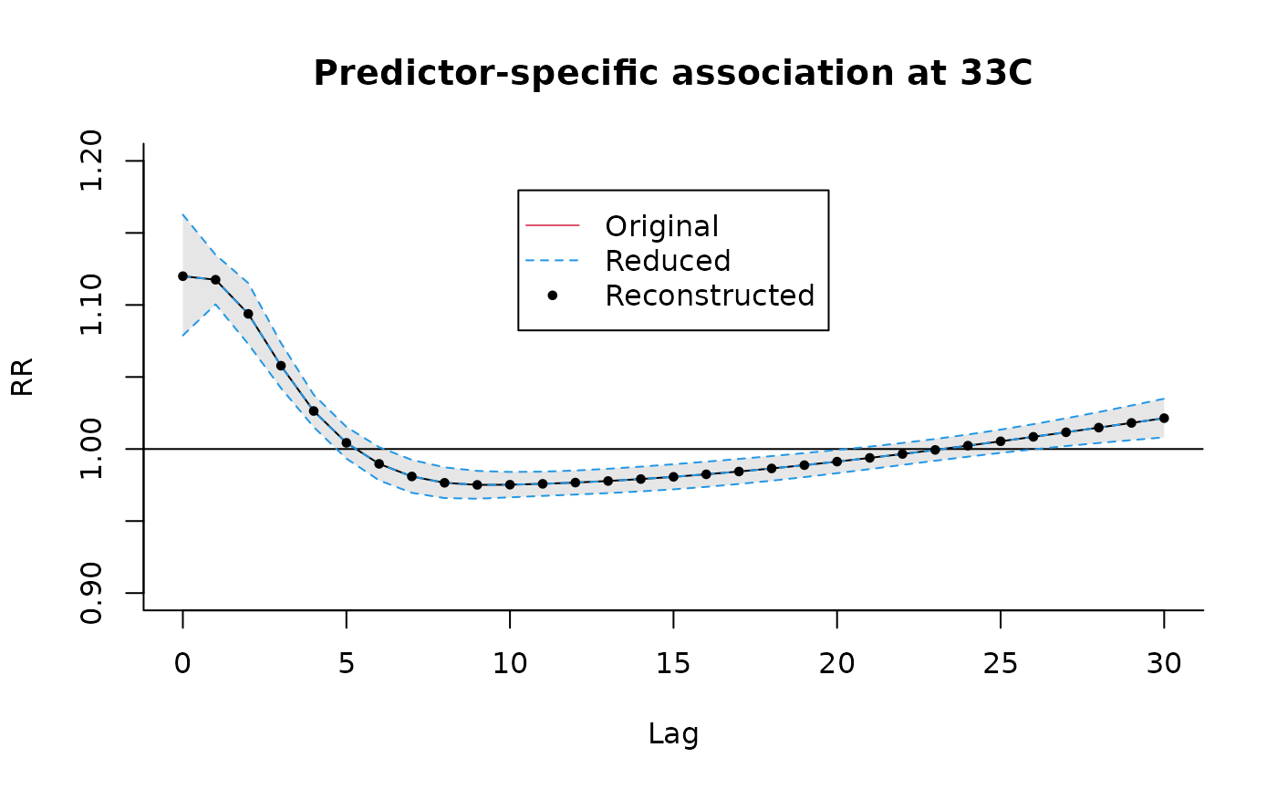
### code chunk number 30: example4plotvar
plot(pred4, "slices",
var = 33, ylab = "RR", ylim = c(0.9, 1.2),
main = "Predictor-specific association at 33C"
)
lines(redvar, ci = "lines", col = 4, lty = 2)
points(pred4b, col = 1, pch = 19, cex = 0.6)
legend("top", c("Original", "Reduced", "Reconstructed"),
col = c(2, 4, 1), lty = c(1:2, NA),
pch = c(NA, NA, 19), pt.cex = 0.6, ins = 0.1
)