Spatial interpolation
spInterp.RdThe irregularly-spaced data are interpolated onto regular latitude-longitude
grids by weighting each station according to its distance or angle from the
center of the search radius cdd.
Arguments
- points
A matrix (N,2) with longitude and latitude of points of data observed
- dat
matrix,
[npoint, ntime], the observed data used to interpolate grid- range
[xmin, xmax, ymin, ymax]- res
the grid resolution (degree)
- fun.weight
function to calculate weight, one of
c("cal_weight", "cal_weight_sf").- wFUN
wFUN_*functions, seewFUN()for details- ...
other parameters to plyr::ldply
- Z
covariates, not used
- weight
predefined weight to speed-up calculation, which is returned by
spInterp()itself.
References
Xavier, A. C., King, C. W., & Scanlon, B. R. (2016). Daily gridded meteorological variables in Brazil (1980-2013). International Journal of Climatology, 36(6), 2644-2659. doi:10.1002/joc.4518
See also
Examples
library(ggplot2)
data(TempBrazil) # Temperature for some poins of Brazil
loc <- TempBrazil[, 1:2] %>% set_names(c("lon", "lat"))
dat <- TempBrazil[, 3] %>% as.matrix() # Vector with observations in points
range <- c(-78, -34, -36, 5)
res = 1
# weight <- weight_adw(loc, range = range, res = 1)
# first example:
r = spInterp_adw(loc, dat, range, res = res, cdd = 450)
print(str(r))
#> List of 3
#> $ weight :Classes ‘data.table’ and 'data.frame': 6349 obs. of 6 variables:
#> ..$ lon : num [1:6349] -55.5 -55.5 -55.5 -54.5 -54.5 -54.5 -53.5 -53.5 -53.5 -52.5 ...
#> ..$ lat : num [1:6349] -34.5 -34.5 -34.5 -34.5 -34.5 -34.5 -34.5 -34.5 -34.5 -34.5 ...
#> ..$ I : int [1:6349] 220 21 213 220 213 21 220 213 21 220 ...
#> ..$ dist : num [1:6349] 224 379 421 151 357 ...
#> ..$ angle: num [1:6349] 60.7 20.6 49.6 42.7 39.4 ...
#> ..$ w : num [1:6349] 0.1573 0.0418 0.0246 0.2879 0.0429 ...
#> ..- attr(*, ".internal.selfref")=<externalptr>
#> $ coord :Classes ‘data.table’ and 'data.frame': 932 obs. of 2 variables:
#> ..$ lon: num [1:932] -73.5 -73.5 -73.5 -73.5 -72.5 -72.5 -72.5 -72.5 -72.5 -72.5 ...
#> ..$ lat: num [1:932] -8.5 -7.5 -6.5 -5.5 -9.5 -8.5 -7.5 -6.5 -5.5 -4.5 ...
#> ..- attr(*, ".internal.selfref")=<externalptr>
#> ..- attr(*, "sorted")= chr [1:2] "lon" "lat"
#> $ predicted: num [1:932, 1] 25 25 25 25 25 ...
#> ..- attr(*, "dimnames")=List of 2
#> .. ..$ : NULL
#> .. ..$ : chr "1"
#> - attr(*, "class")= chr "spInterp"
#> NULL
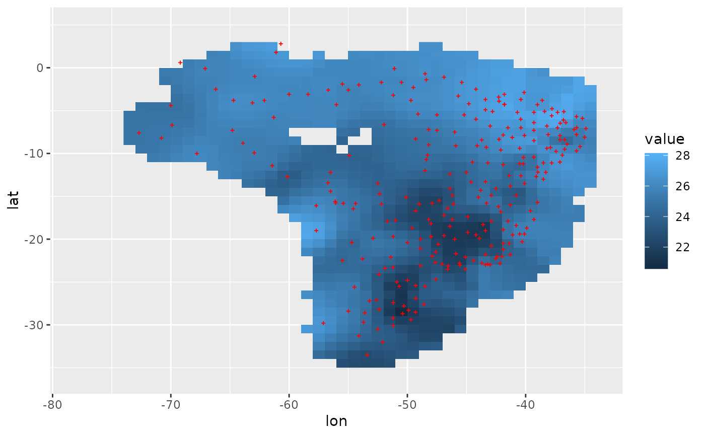
df = r %$% cbind(coord, value = predicted[, 1])
ggplot(df, aes(lon, lat)) +
geom_raster(aes(fill = value)) +
geom_point(data = loc, size = 0.5, shape = 3, color = "red") +
lims(x = range[1:2], y = range[3:4])
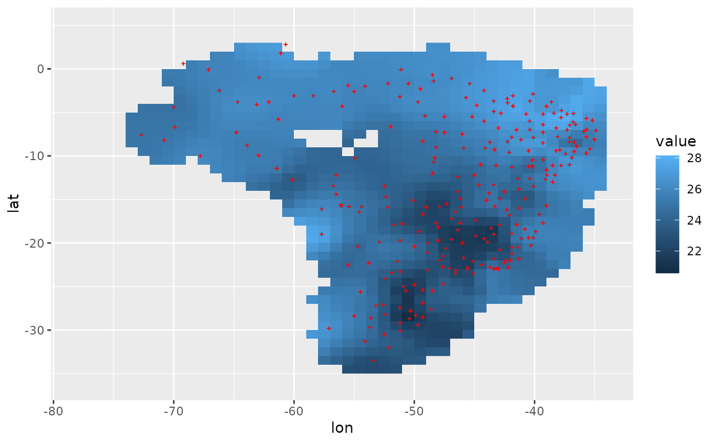 # second example: use sf as backend, but of low computing efficiency, 100 times slower
r_sf = spInterp_adw(loc, dat, range, res = res, cdd = 450, fun.weight = "cal_weight_sf")
df_sf = r_sf %$% cbind(coord, value = predicted[, 1])
ggplot(df_sf, aes(lon, lat)) +
geom_raster(aes(fill = value)) +
geom_point(data = loc, size = 0.5, shape = 3, color = "red") +
lims(x = range[1:2], y = range[3:4])
# second example: use sf as backend, but of low computing efficiency, 100 times slower
r_sf = spInterp_adw(loc, dat, range, res = res, cdd = 450, fun.weight = "cal_weight_sf")
df_sf = r_sf %$% cbind(coord, value = predicted[, 1])
ggplot(df_sf, aes(lon, lat)) +
geom_raster(aes(fill = value)) +
geom_point(data = loc, size = 0.5, shape = 3, color = "red") +
lims(x = range[1:2], y = range[3:4])
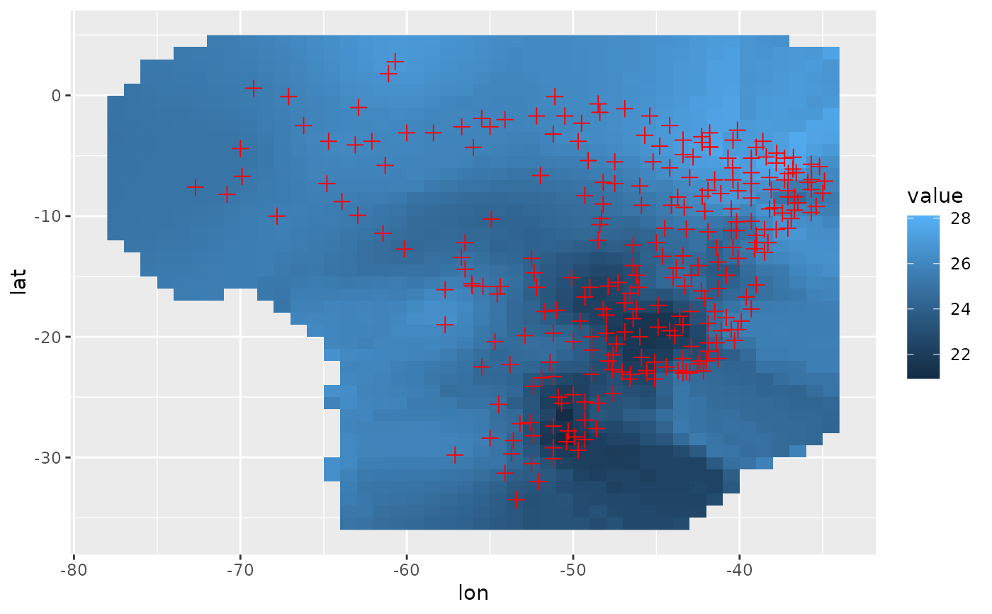
 # third example: use a large `cdd`, set `cdd = 1000`
r = spInterp_adw(loc, dat, range, res = res, cdd = 1000)
df = r %$% cbind(coord, value = predicted[, 1])
ggplot(df, aes(lon, lat)) +
geom_raster(aes(fill = value)) +
geom_point(data = loc, size = 2.5, shape = 3, color = "red") +
lims(x = range[1:2], y = range[3:4])
# third example: use a large `cdd`, set `cdd = 1000`
r = spInterp_adw(loc, dat, range, res = res, cdd = 1000)
df = r %$% cbind(coord, value = predicted[, 1])
ggplot(df, aes(lon, lat)) +
geom_raster(aes(fill = value)) +
geom_point(data = loc, size = 2.5, shape = 3, color = "red") +
lims(x = range[1:2], y = range[3:4])