geom_raster_filled
geom_raster_filled.Rdstat_levels() is the geom-agnostic engine of the level-binning family. It
discretizes the continuous aesthetic z into a factor level via
base::cut() and, by default, maps that level to fill so it can drive
any geom (point, raster, tile, ...). stat_raster_levels() and
stat_point_levels() are thin subclasses that reuse this binning logic and
only change which aesthetic level is mapped to.
geom_raster_filled(
  mapping = NULL,
  data = NULL,
  stat = "raster_levels",
  position = "identity",
  ...,
  breaks = NULL,
  hjust = 0.5,
  vjust = 0.5,
  interpolate = FALSE,
  na.rm = FALSE,
  show.legend = NA,
  inherit.aes = TRUE
)

stat_raster_levels(
  mapping = NULL,
  data = NULL,
  geom = "raster",
  position = "identity",
  ...,
  breaks = NULL,
  na.rm = FALSE,
  show.legend = NA,
  inherit.aes = TRUE
)

stat_levels(
  mapping = NULL,
  data = NULL,
  geom = "point",
  position = "identity",
  ...,
  breaks = NULL,
  include.lowest = FALSE,
  na.rm = FALSE,
  show.legend = NA,
  inherit.aes = TRUE
)
Arguments
- mapping
Set of aesthetic mappings created by
aes(). If specified andinherit.aes = TRUE(the default), it is combined with the default mapping at the top level of the plot. You must supplymappingif there is no plot mapping.- data
The data to be displayed in this layer. There are three options:
If
NULL, the default, the data is inherited from the plot data as specified in the call toggplot().A
data.frame, or other object, will override the plot data. All objects will be fortified to produce a data frame. Seefortify()for which variables will be created.A
functionwill be called with a single argument, the plot data. The return value must be adata.frame, and will be used as the layer data. Afunctioncan be created from aformula(e.g.~ head(.x, 10)).- stat
The statistical transformation to use on the data for this layer. When using a
geom_*()function to construct a layer, thestatargument can be used to override the default coupling between geoms and stats. Thestatargument accepts the following:A
Statggproto subclass, for exampleStatCount.A string naming the stat. To give the stat as a string, strip the function name of the
stat_prefix. For example, to usestat_count(), give the stat as"count".For more information and other ways to specify the stat, see the layer stat documentation.
- position
A position adjustment to use on the data for this layer. This can be used in various ways, including to prevent overplotting and improving the display. The
positionargument accepts the following:The result of calling a position function, such as
position_jitter(). This method allows for passing extra arguments to the position.A string naming the position adjustment. To give the position as a string, strip the function name of the
position_prefix. For example, to useposition_jitter(), give the position as"jitter".For more information and other ways to specify the position, see the layer position documentation.
- ...
Other arguments passed on to
layer()'sparamsargument. These arguments broadly fall into one of 4 categories below. Notably, further arguments to thepositionargument, or aesthetics that are required can not be passed through.... Unknown arguments that are not part of the 4 categories below are ignored.Static aesthetics that are not mapped to a scale, but are at a fixed value and apply to the layer as a whole. For example,
colour = "red"orlinewidth = 3. The geom's documentation has an Aesthetics section that lists the available options. The 'required' aesthetics cannot be passed on to theparams. Please note that while passing unmapped aesthetics as vectors is technically possible, the order and required length is not guaranteed to be parallel to the input data.When constructing a layer using a
stat_*()function, the...argument can be used to pass on parameters to thegeompart of the layer. An example of this isstat_density(geom = "area", outline.type = "both"). The geom's documentation lists which parameters it can accept.Inversely, when constructing a layer using a
geom_*()function, the...argument can be used to pass on parameters to thestatpart of the layer. An example of this isgeom_area(stat = "density", adjust = 0.5). The stat's documentation lists which parameters it can accept.The
key_glyphargument oflayer()may also be passed on through.... This can be one of the functions described as key glyphs, to change the display of the layer in the legend.
- breaks
Numeric vector of break points passed to
base::cut()to binzinto discrete levels. WhenNULL(the default),pretty(z, 7)is used. To capture values below the smallest / above the largest break, include-Inf/Infinbreaks(e.g.c(-Inf, 2, 4, 6, Inf)); otherwise out-of-range values becomeNAand are dropped. This is the opposite of the continuousscale_*_stepsn()path, which requires finite breaks.- hjust, vjust
horizontal and vertical justification of the grob. Each justification value should be a number between 0 and 1. Defaults to 0.5 for both, centering each pixel over its data location.
- interpolate
If
TRUEinterpolate linearly, ifFALSE(the default) don't interpolate.- na.rm
If
FALSE, the default, missing values are removed with a warning. IfTRUE, missing values are silently removed.- show.legend
logical. Should this layer be included in the legends?
NA, the default, includes if any aesthetics are mapped.FALSEnever includes, andTRUEalways includes. It can also be a named logical vector to finely select the aesthetics to display. To include legend keys for all levels, even when no data exists, useTRUE. IfNA, all levels are shown in legend, but unobserved levels are omitted.- inherit.aes
If
FALSE, overrides the default aesthetics, rather than combining with them. This is most useful for helper functions that define both data and aesthetics and shouldn't inherit behaviour from the default plot specification, e.g.annotation_borders().- geom
The geometric object to use to display the data for this layer. When using a
stat_*()function to construct a layer, thegeomargument can be used to override the default coupling between stats and geoms. Thegeomargument accepts the following:A
Geomggproto subclass, for exampleGeomPoint.A string naming the geom. To give the geom as a string, strip the function name of the
geom_prefix. For example, to usegeom_point(), give the geom as"point".For more information and other ways to specify the geom, see the layer geom documentation.
- include.lowest
Logical, passed to
base::cut(). IfTRUE, a value equal to the lowest break is included in the first interval. This only rescues the boundary value itself; it does not capture values truly below the lowest break (use-Inffor that).
Computed variables
levelthe factor produced by
cut(z, breaks); map it to an aesthetic withafter_stat(level).
Aesthetics
stat_levels() requires the z aesthetic and, by default, maps the
computed level to fill. To colour points instead, either map it
explicitly with aes(colour = after_stat(level)) and silence the unused
default fill legend via guides(fill = "none"), or use the dedicated
geom_point_levels() / stat_point_levels(), which map only colour.
See also
geom_raster_filled(), geom_point_levels(),
stat_raster_levels(), stat_point_levels(), base::cut()
Examples
library(rcolors)
library(ggplot2)
library(magrittr)
df = data.frame(x = 1:10, y = 1:10, z = 1:10)
brks <- c(2, 4, 6, 8) %>% c(-Inf, ., Inf) # 这里要包含
nbrk <- length(brks) - 1
cols = get_color(rcolors$amwg256, nbrk)
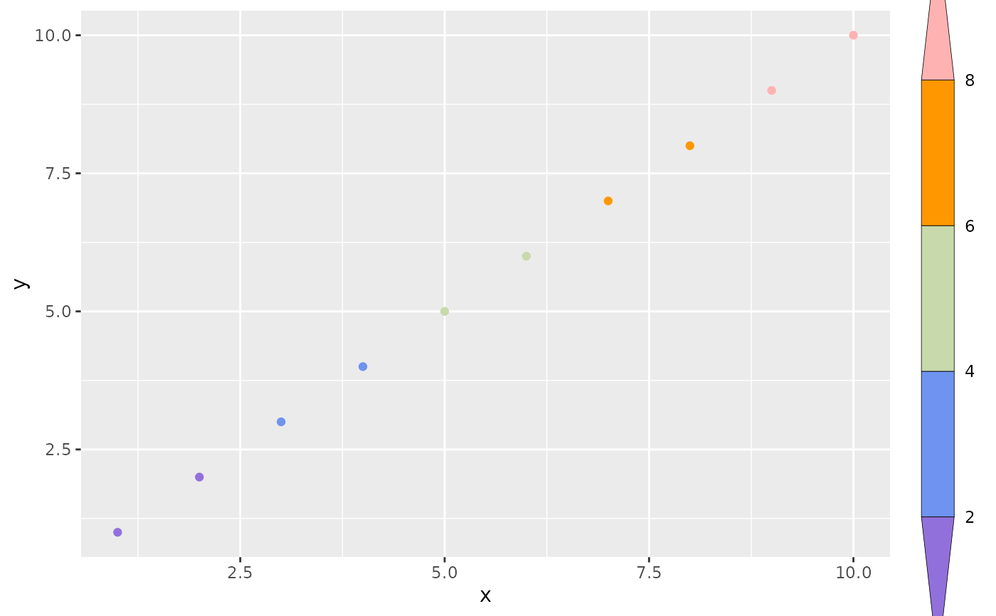
ggplot(df, aes(x, y, z = x)) +
stat_levels(aes(color = after_stat(level)), breaks = brks, geom = "point") +
scale_color_manual(
values = cols,
guide = guide_coloursteps2(title = "lgd", barheight = unit(0.8, "npc"))
) +
guides(fill = "none")
 ## another option: use `scale_color_stepsn`
# example 2
# NOTE: `scale_*_stepsn` is a *continuous* binned scale, so `breaks` must be
# finite. Passing -Inf/Inf makes the open-ended end bins rescale to a
# non-finite value -> palette returns NA -> drawn as grey (na.value). Drop the
# infinite breaks here; the open-ended triangles are still drawn by
# `guide_coloursteps2()` (which always renders triangle ends), so no semantics
# are lost. Note the bin colours are *interpolated* along the gradient and thus
# only approximate `cols`; for exact per-level colours use the discrete `cut`
# path above (stat_levels + scale_color_manual).
ggplot(df, aes(x, y, color = x)) +
geom_point() +
scale_color_stepsn(
colors = cols,
breaks = brks[is.finite(brks)],
guide = guide_coloursteps2(title = "lgd")
) +
theme(
legend.title = element_blank(),
legend.margin = margin(l = -2)
)
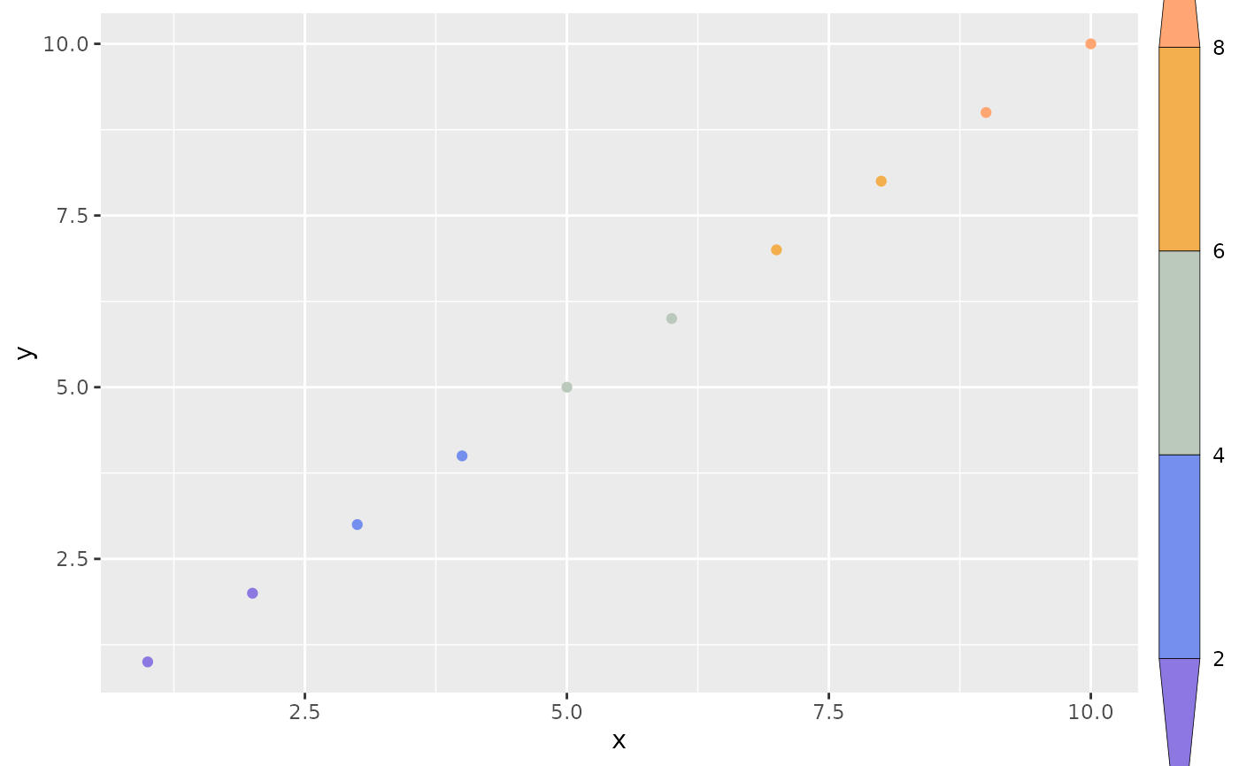
## another option: use `scale_color_stepsn`
# example 2
# NOTE: `scale_*_stepsn` is a *continuous* binned scale, so `breaks` must be
# finite. Passing -Inf/Inf makes the open-ended end bins rescale to a
# non-finite value -> palette returns NA -> drawn as grey (na.value). Drop the
# infinite breaks here; the open-ended triangles are still drawn by
# `guide_coloursteps2()` (which always renders triangle ends), so no semantics
# are lost. Note the bin colours are *interpolated* along the gradient and thus
# only approximate `cols`; for exact per-level colours use the discrete `cut`
# path above (stat_levels + scale_color_manual).
ggplot(df, aes(x, y, color = x)) +
geom_point() +
scale_color_stepsn(
colors = cols,
breaks = brks[is.finite(brks)],
guide = guide_coloursteps2(title = "lgd")
) +
theme(
legend.title = element_blank(),
legend.margin = margin(l = -2)
)
 # example 3
df <- expand.grid(X1 = 1:10, X2 = 1:10)
df$value <- df$X1 * df$X2
brks = c(10, 15, 25, 50)
nbrk <- length(brks) + 1
cols = get_color(rcolors$amwg256, nbrk)
# This can be changed with the `even.steps` argument
ggplot(df, aes(X1, X2)) +
geom_tile(aes(fill = value)) +
scale_fill_stepsn(
colors = cols, breaks = brks,
guide = guide_colorsteps2()
) +
theme(
legend.title = element_blank(),
legend.margin = margin(l = -2)
)
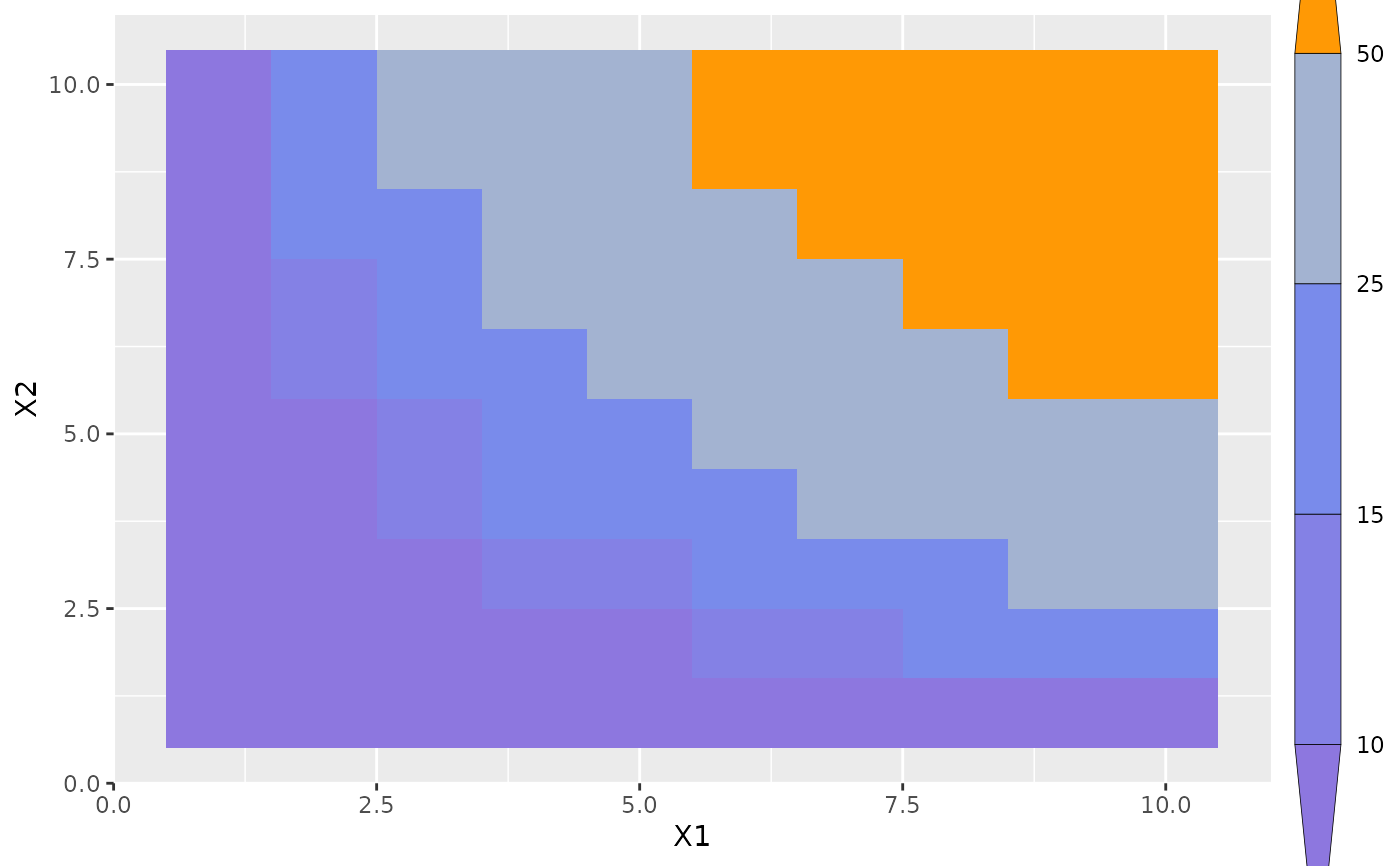
# example 3
df <- expand.grid(X1 = 1:10, X2 = 1:10)
df$value <- df$X1 * df$X2
brks = c(10, 15, 25, 50)
nbrk <- length(brks) + 1
cols = get_color(rcolors$amwg256, nbrk)
# This can be changed with the `even.steps` argument
ggplot(df, aes(X1, X2)) +
geom_tile(aes(fill = value)) +
scale_fill_stepsn(
colors = cols, breaks = brks,
guide = guide_colorsteps2()
) +
theme(
legend.title = element_blank(),
legend.margin = margin(l = -2)
)